CPSC 330 Python notes

About this document

This document contains some Python lecture materials from the 1st offering of CPSC 330. We have decided to stop allocated lecture time to this topic and instead have this as reference material.

import numpy as np
import pandas as pd

Plotting with matplotlib

• We will use matplotlib as our plotting library.

• For those familiar with MATLAB, this package is based on MATLAB plotting.

• To use matplotlib, we first import it:

import matplotlib.pyplot as plt

• We can now use functions in plt to plot things:

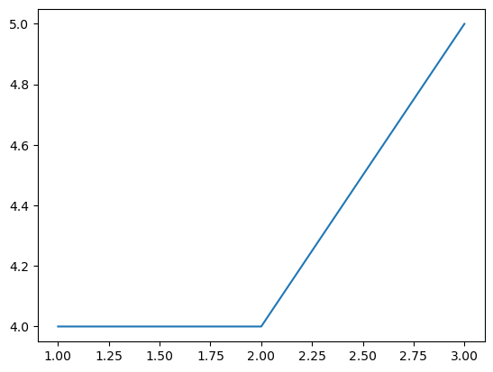
x = [1,2,3]
y = [4,4,5]
plt.plot(x,y)

[<matplotlib.lines.Line2D at 0x16835f3d0>]

• You will often see me put a semicolon at the end of a line.

• This is only relevant to Jupyter; it suppresses the line of “output”..

plt.plot(x,y);

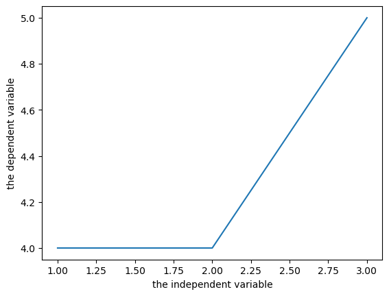
• In your homework assignments, at a minimum, you should have axis labels for every figure that you submit.

plt.plot(x,y)
plt.xlabel("the independent variable")
plt.ylabel("the dependent variable");

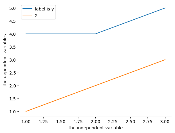
• If you are plotting multiple curves, make sure you include a legend!

plt.plot(x,y, label="label is y")
plt.plot(x,x, label="x")
plt.xlabel("the independent variable")
plt.ylabel("the dependent variables")
plt.legend();

• You will likely need to visit the matplotlib.pyplot documentation when trying to do other things.

• When you save an .ipynb file, the output, including plots, is stored in the file.

  • This is a hassle for git.

  • But it’s also convenient.

  • This is how you will submit plots.

Numpy arrays

Basic numpy is covered in the posted videos, you are expected to have a basic knowledge of numpy.

x = np.zeros(4)
x

array([0., 0., 0., 0.])

y = np.ones(4)

x+y

array([1., 1., 1., 1.])

z = np.random.rand(2,3)
z

array([[0.15643684, 0.42108204, 0.81939978],
       [0.65537007, 0.50742398, 0.97737839]])

z[0,1]

0.42108204325103504

Numpy array shapes

One of the most confusing things about numpy: what I call a “1-D array” can have 3 possible shapes:

x = np.ones(5)
print(x)
print("size:", x.size)
print("ndim:", x.ndim)
print("shape:",x.shape)

[1. 1. 1. 1. 1.]
size: 5
ndim: 1
shape: (5,)

y = np.ones((1,5))
print(y)
print("size:", y.size)
print("ndim:", y.ndim)
print("shape:",y.shape)

[[1. 1. 1. 1. 1.]]
size: 5
ndim: 2
shape: (1, 5)

z = np.ones((5,1))
print(z)
print("size:", z.size)
print("ndim:", z.ndim)
print("shape:",z.shape)

[[1.]
 [1.]
 [1.]
 [1.]
 [1.]]
size: 5
ndim: 2
shape: (5, 1)

np.array_equal(x,y)

False

np.array_equal(x,z)

False

np.array_equal(y,z)

False

Broadcasting in numpy

• Arrays with different sizes cannot be directly used in arithmetic operations.

• Broadcasting describes how numpy treats arrays with different shapes during arithmetic operations.

• The idea is to vectorize operations to avoid loops and speed up the code.

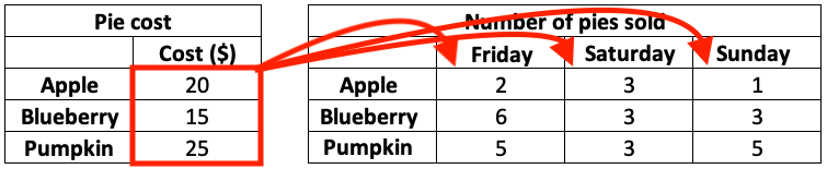
• Example: I sell pies on the weekends.

• I sell 3 types of pies at different prices, and I sold the following number of each pie last weekend.

• I want to know how much money I made per pie type per day.

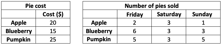
cost = np.array([20, 15, 25])
print("Pie cost:")
print(cost.reshape(3,1))
sales = np.array([[2, 3, 1],
                  [6, 3, 3],
                  [5, 3, 5]])
print("\nPie sales (#):")
print(sales)

Pie cost:
[[20]
 [15]
 [25]]

Pie sales (#):
[[2 3 1]
 [6 3 3]
 [5 3 5]]

• How can we multiply these two arrays together?

Slowest method: nested loop

total = np.zeros((3, 3))
for i in range(3):
    for j in range(3):
        total[i,j] = cost[i] * sales[i,j]
total

array([[ 40.,  60.,  20.],
       [ 90.,  45.,  45.],
       [125.,  75., 125.]])

Faster method: vectorize the loop over rows

total = np.zeros((3, 3))
for j in range(3):
    total[:,j] = cost * sales[:,j]
total

array([[ 40.,  60.,  20.],
       [ 90.,  45.,  45.],
       [125.,  75., 125.]])

No-loop method: make them the same size, and multiply element-wise

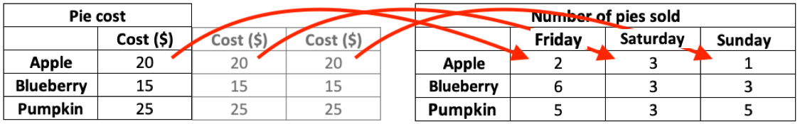
cost_rep = np.repeat(cost[:,np.newaxis], 3, axis=1)
cost_rep

array([[20, 20, 20],
       [15, 15, 15],
       [25, 25, 25]])

cost_rep * sales

array([[ 40,  60,  20],
       [ 90,  45,  45],
       [125,  75, 125]])

• What is np.newaxis?

• It changes the shape:

cost.shape

(3,)

cost[:,np.newaxis].shape

(3, 1)

cost.reshape(3,1).shape # the name thing

(3, 1)

cost[np.newaxis].shape

(1, 3)

Fastest method: broadcasting

cost[:,np.newaxis] * sales

array([[ 40,  60,  20],
       [ 90,  45,  45],
       [125,  75, 125]])

• numpy does the equivalent of np.repeat() for you - no need to do it explicitly

• It is debatable whether this code is more readable, but it is definitely faster.

When can we use broadcasting?

Say we want to broadcast the following two arrays:

arr1 = np.arange(3)
arr2 = np.ones((5))

arr1

array([0, 1, 2])

arr2

array([1., 1., 1., 1., 1.])

arr1.shape

(3,)

arr2.shape

(5,)

• The broadcast will fail because the arrays are not compatible…

arr1 + arr2

---------------------------------------------------------------------------
ValueError                                Traceback (most recent call last)
Cell In[33], line 1
----> 1 arr1 + arr2

ValueError: operands could not be broadcast together with shapes (3,) (5,) 

• We can facilitate this broadcast by adding a dimension using np.newaxis.

• np.newaxis increases the dimension of an array by one dimension.

arr1.shape

(3,)

arr1 = arr1[:, np.newaxis]

arr1.shape

(3, 1)

arr2 = arr2[np.newaxis]

arr2.shape

(1, 5)

arr1 + arr2

array([[1., 1., 1., 1., 1.],
       [2., 2., 2., 2., 2.],
       [3., 3., 3., 3., 3.]])

• the opposite, reducing a dimension, can be achieved by np.squeeze()

arr1.shape

(3, 1)

np.squeeze(arr1).shape

(3,)

The rules of broadcasting:

• NumPy compares arrays one dimension at a time. It starts with the trailing dimensions, and works its way to the first dimensions.

• dimensions are compatible if:

  • they are equal, or

  • one of them is 1.

• Use the code below to test out array compatibitlity

a = np.ones((5,1))
b = np.ones((1,3))
print(f"The shape of a is: {a.shape}")
print(f"The shape of b is: {b.shape}")
try:
    print(f"The shape of a + b is: {(a + b).shape}")
except:
    print(f"ERROR: arrays are NOT broadcast compatible!")

The shape of a is: (5, 1)
The shape of b is: (1, 3)
The shape of a + b is: (5, 3)

Introduction to pandas

• The most popular Python library for tabular data structures

import pandas as pd

Pandas Series

• A Series is like a NumPy array but with labels

• 1-dimensional

• Can be created from a list, ndarray or dictionary using pd.Series()

• Labels may be integers or strings

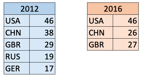
Here are two series of gold medal counts for the 2012 and 2016 Olympics:

pd.Series()

Series([], dtype: float64)

s1 = pd.Series(data = [46, 38, 29, 19, 17],
               index = ['USA','CHN','GBR','RUS','GER'])
s1

USA    46
CHN    38
GBR    29
RUS    19
GER    17
dtype: int64

s2 = pd.Series([46, 26, 27],
               ['USA', 'CHN', 'GBR'])
s2

USA    46
CHN    26
GBR    27
dtype: int64

• Like ndarrays we use square brackets [] to index a series

• BUT, Series can be indexed by an integer location OR a label

s1

USA    46
CHN    38
GBR    29
RUS    19
GER    17
dtype: int64

s1.iloc[0]

46

s1.iloc[1]

38

s1["USA"]

46

s1["USA":"RUS"]

USA    46
CHN    38
GBR    29
RUS    19
dtype: int64

Do we expect these two series to be compatible for broadcasting?

s1

USA    46
CHN    38
GBR    29
RUS    19
GER    17
dtype: int64

s2

USA    46
CHN    26
GBR    27
dtype: int64

print(f"The shape of s1 is: {s1.shape}")
print(f"The shape of s2 is: {s2.shape}")

The shape of s1 is: (5,)
The shape of s2 is: (3,)

s1 + s2

CHN    64.0
GBR    56.0
GER     NaN
RUS     NaN
USA    92.0
dtype: float64

• Unlike ndarrays operations between Series (+, -, /, *) align values based on their LABELS

• The result index will be the sorted union of the two indexes

Pandas DataFrames

• The primary Pandas data structure

• Really just a bunch of Series (with the same index labels) stuck together

• Made using pd.DataFrame()

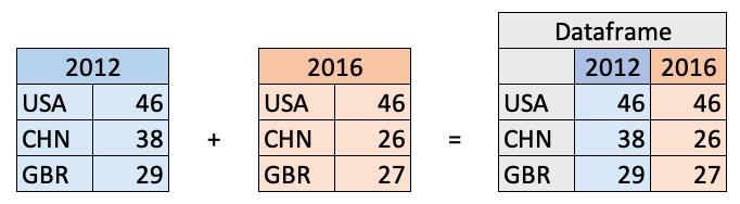
Creating a DataFrame with a numpy array

d = np.array([[46, 46],
              [38, 26],
              [29, 27]])
c = ['2012', '2016']
i = ['USA', 'CHN', 'GBR']
df = pd.DataFrame(data=d, index=i, columns=c)
df

	2012	2016
USA	46	46
CHN	38	26
GBR	29	27

(optional) Creating a DataFrame with a dictionary

d = {'2012': [46, 38, 29],
     '2016': [46, 26, 27]}
i = ['USA', 'CHN', 'GBR']
df = pd.DataFrame(d, i)
df

	2012	2016
USA	46	46
CHN	38	26
GBR	29	27

Indexing Dataframes

• There are three main ways to index a DataFrame:

  1. [] (slice for rows, label for columns)

  2. .loc[]

  3. .iloc[]

df

	2012	2016
USA	46	46
CHN	38	26
GBR	29	27

[] notation

• you can index columns by single labels or lists of labels

df['2012']

USA    46
CHN    38
GBR    29
Name: 2012, dtype: int64

type(df['2012'])

pandas.core.series.Series

type(['2012', '2016'])

list

df[['2012', '2016']]

	2012	2016
USA	46	46
CHN	38	26
GBR	29	27

(optional) you can also index rows with [], but you can only index rows with slices

df["CHN":"GBR"]

	2012	2016
CHN	38	26
GBR	29	27

# df["USA"] # doesn't work

df[:"USA"] # does work

	2012	2016
USA	46	46

• this is a little unintuitive, so pandas created two other ways to index a dataframe:

• for indexing with integers: df.iloc[]

• for indexing with labels: df.loc[]

df

	2012	2016
USA	46	46
CHN	38	26
GBR	29	27

df.iloc[1]

2012    38
2016    26
Name: CHN, dtype: int64

df.iloc[2,1]

27

df.loc['CHN']

2012    38
2016    26
Name: CHN, dtype: int64

df.loc['GBR', '2016']

27

df.loc[['USA', 'GBR'], ['2012']]

	2012
USA	46
GBR	29

df.index

Index(['USA', 'CHN', 'GBR'], dtype='object')

df.columns

Index(['2012', '2016'], dtype='object')

#df.loc[df.index[0], '2016']

#df.loc['USA', df.columns[0]]

Indexing cheatsheet

• [] accepts slices for row indexing or labels (single or list) for column indexing

• .iloc[] accepts integers for row/column indexing, and can be single values or lists

• .loc[] accepts labels for row/column indexing, and can be single values or lists

• for integer row/named column: df.loc[df.index[#], 'labels']

• for named row/integer column: df.loc['labels', df.columns[#]]

Break (5 min)

Reading from .csv

• Most of the time you will be loading .csv files for use in pandas using pd.read_csv()

• Example dataset: a colleague’s cycling commute to/from UBC everyday

path = 'data/cycling_data.csv'

pd.read_csv(path, index_col=0, parse_dates=True).head()

	Name	Type	Time	Distance	Comments
Date
2019-09-10 00:13:04	Afternoon Ride	Ride	2084	12.62	Rain
2019-09-10 13:52:18	Morning Ride	Ride	2531	13.03	rain
2019-09-11 00:23:50	Afternoon Ride	Ride	1863	12.52	Wet road but nice weather
2019-09-11 14:06:19	Morning Ride	Ride	2192	12.84	Stopped for photo of sunrise
2019-09-12 00:28:05	Afternoon Ride	Ride	1891	12.48	Tired by the end of the week

Reading from url

• you may also want to read directly from an url at times

• pd.read_csv() accepts urls as input

url = 'https://raw.githubusercontent.com/TomasBeuzen/toy-datasets/master/wine_1.csv'
pd.read_csv(url)

	Bottle	Grape	Origin	Alcohol	pH	Colour	Aroma
0	1	Chardonnay	Australia	14.23	3.51	White	Floral
1	2	Pinot Grigio	Italy	13.20	3.30	White	Fruity
2	3	Pinot Blanc	France	13.16	3.16	White	Citrus
3	4	Shiraz	Chile	14.91	3.39	Red	Berry
4	5	Malbec	Argentina	13.83	3.28	Red	Fruity

Reading from other formats

• pd.read_excel()

• pd.read_html()

• pd.read_json()

• etc

Dataframe summaries

df = pd.read_csv('data/cycling_data.csv')
df.head()

	Date	Name	Type	Time	Distance	Comments
0	10 Sep 2019, 00:13:04	Afternoon Ride	Ride	2084	12.62	Rain
1	10 Sep 2019, 13:52:18	Morning Ride	Ride	2531	13.03	rain
2	11 Sep 2019, 00:23:50	Afternoon Ride	Ride	1863	12.52	Wet road but nice weather
3	11 Sep 2019, 14:06:19	Morning Ride	Ride	2192	12.84	Stopped for photo of sunrise
4	12 Sep 2019, 00:28:05	Afternoon Ride	Ride	1891	12.48	Tired by the end of the week

df.info()

<class 'pandas.core.frame.DataFrame'>
RangeIndex: 33 entries, 0 to 32
Data columns (total 6 columns):
Date        33 non-null object
Name        33 non-null object
Type        33 non-null object
Time        33 non-null int64
Distance    31 non-null float64
Comments    33 non-null object
dtypes: float64(1), int64(1), object(4)
memory usage: 1.7+ KB

df.describe(include='all')

	Date	Name	Type	Time	Distance	Comments
count	33	33	33	33.000000	31.000000	33
unique	33	2	1	NaN	NaN	25
top	26 Sep 2019, 13:42:43	Afternoon Ride	Ride	NaN	NaN	Feeling good
freq	1	17	33	NaN	NaN	3
mean	NaN	NaN	NaN	3512.787879	12.667419	NaN
std	NaN	NaN	NaN	8003.309233	0.428618	NaN
min	NaN	NaN	NaN	1712.000000	11.790000	NaN
25%	NaN	NaN	NaN	1863.000000	12.480000	NaN
50%	NaN	NaN	NaN	2118.000000	12.620000	NaN
75%	NaN	NaN	NaN	2285.000000	12.750000	NaN
max	NaN	NaN	NaN	48062.000000	14.570000	NaN

Renaming columns with df.rename()

df.head()

	Date	Name	Type	Time	Distance	Comments
0	10 Sep 2019, 00:13:04	Afternoon Ride	Ride	2084	12.62	Rain
1	10 Sep 2019, 13:52:18	Morning Ride	Ride	2531	13.03	rain
2	11 Sep 2019, 00:23:50	Afternoon Ride	Ride	1863	12.52	Wet road but nice weather
3	11 Sep 2019, 14:06:19	Morning Ride	Ride	2192	12.84	Stopped for photo of sunrise
4	12 Sep 2019, 00:28:05	Afternoon Ride	Ride	1891	12.48	Tired by the end of the week

• we can rename specific columns using df.rename()

{"Comments": "Notes"}

{'Comments': 'Notes'}

type({"Comments": "Notes"})

dict

df = df.rename(columns={"Comments": "Notes"})
df.head()

	Date	Name	Type	Time	Distance	Notes
0	10 Sep 2019, 00:13:04	Afternoon Ride	Ride	2084	12.62	Rain
1	10 Sep 2019, 13:52:18	Morning Ride	Ride	2531	13.03	rain
2	11 Sep 2019, 00:23:50	Afternoon Ride	Ride	1863	12.52	Wet road but nice weather
3	11 Sep 2019, 14:06:19	Morning Ride	Ride	2192	12.84	Stopped for photo of sunrise
4	12 Sep 2019, 00:28:05	Afternoon Ride	Ride	1891	12.48	Tired by the end of the week

• there are two options for making permanent dataframe changes:

  • 1. set the argument inplace=True, e.g., df.rename(..., inplace=True)

  • 2. re-assign, e.g., df = df.rename(...)

df.rename(columns={"Comments": "Notes"}, inplace=True) # inplace
df = df.rename(columns={"Comments": "Notes"}) # re-assign

NOTE:

• the pandas team discourages the use of inplace for a few reasons

• mostly because not all functions have the argument, hides memory copying, leads to hard-to-find bugs

• it is recommend to re-assign (method 2 above)

• we can also change all columns at once using a list

df.columns = ['col1', 'col2', 'col3', 'col4', 'col5', 'col6']
df.head()

	col1	col2	col3	col4	col5	col6
0	10 Sep 2019, 00:13:04	Afternoon Ride	Ride	2084	12.62	Rain
1	10 Sep 2019, 13:52:18	Morning Ride	Ride	2531	13.03	rain
2	11 Sep 2019, 00:23:50	Afternoon Ride	Ride	1863	12.52	Wet road but nice weather
3	11 Sep 2019, 14:06:19	Morning Ride	Ride	2192	12.84	Stopped for photo of sunrise
4	12 Sep 2019, 00:28:05	Afternoon Ride	Ride	1891	12.48	Tired by the end of the week

Adding/removing columns with [] and drop()

df = pd.read_csv('data/cycling_data.csv')
df.head()

	Date	Name	Type	Time	Distance	Comments
0	10 Sep 2019, 00:13:04	Afternoon Ride	Ride	2084	12.62	Rain
1	10 Sep 2019, 13:52:18	Morning Ride	Ride	2531	13.03	rain
2	11 Sep 2019, 00:23:50	Afternoon Ride	Ride	1863	12.52	Wet road but nice weather
3	11 Sep 2019, 14:06:19	Morning Ride	Ride	2192	12.84	Stopped for photo of sunrise
4	12 Sep 2019, 00:28:05	Afternoon Ride	Ride	1891	12.48	Tired by the end of the week

• adding a single column

df['Speed'] = 3.14159265358979323
df.head()

	Date	Name	Type	Time	Distance	Comments	Speed
0	10 Sep 2019, 00:13:04	Afternoon Ride	Ride	2084	12.62	Rain	3.141593
1	10 Sep 2019, 13:52:18	Morning Ride	Ride	2531	13.03	rain	3.141593
2	11 Sep 2019, 00:23:50	Afternoon Ride	Ride	1863	12.52	Wet road but nice weather	3.141593
3	11 Sep 2019, 14:06:19	Morning Ride	Ride	2192	12.84	Stopped for photo of sunrise	3.141593
4	12 Sep 2019, 00:28:05	Afternoon Ride	Ride	1891	12.48	Tired by the end of the week	3.141593

• dropping a column

df = df.drop(columns="Speed")
df.head()

	Date	Name	Type	Time	Distance	Comments
0	10 Sep 2019, 00:13:04	Afternoon Ride	Ride	2084	12.62	Rain
1	10 Sep 2019, 13:52:18	Morning Ride	Ride	2531	13.03	rain
2	11 Sep 2019, 00:23:50	Afternoon Ride	Ride	1863	12.52	Wet road but nice weather
3	11 Sep 2019, 14:06:19	Morning Ride	Ride	2192	12.84	Stopped for photo of sunrise
4	12 Sep 2019, 00:28:05	Afternoon Ride	Ride	1891	12.48	Tired by the end of the week

• we can also add/drop multiple columns at a time

df = df.drop(columns=['Type', 'Time'])
df.head()

	Date	Name	Distance	Comments
0	10 Sep 2019, 00:13:04	Afternoon Ride	12.62	Rain
1	10 Sep 2019, 13:52:18	Morning Ride	13.03	rain
2	11 Sep 2019, 00:23:50	Afternoon Ride	12.52	Wet road but nice weather
3	11 Sep 2019, 14:06:19	Morning Ride	12.84	Stopped for photo of sunrise
4	12 Sep 2019, 00:28:05	Afternoon Ride	12.48	Tired by the end of the week

Adding/removing rows with [] and drop()

df = pd.read_csv('data/cycling_data.csv')
df.tail()

	Date	Name	Type	Time	Distance	Comments
28	4 Oct 2019, 01:08:08	Afternoon Ride	Ride	1870	12.63	Very tired, riding into the wind
29	9 Oct 2019, 13:55:40	Morning Ride	Ride	2149	12.70	Really cold! But feeling good
30	10 Oct 2019, 00:10:31	Afternoon Ride	Ride	1841	12.59	Feeling good after a holiday break!
31	10 Oct 2019, 13:47:14	Morning Ride	Ride	2463	12.79	Stopped for photo of sunrise
32	11 Oct 2019, 00:16:57	Afternoon Ride	Ride	1843	11.79	Bike feeling tight, needs an oil and pump

last_row = df.iloc[-1]
last_row

Date                            11 Oct 2019, 00:16:57
Name                                   Afternoon Ride
Type                                             Ride
Time                                             1843
Distance                                        11.79
Comments    Bike feeling tight, needs an oil and pump
Name: 32, dtype: object

df.shape

(optional) We can add the row to the end of the dataframe using df.append()

df = df.append(last_row)
df.tail()

	Date	Name	Type	Time	Distance	Comments
29	9 Oct 2019, 13:55:40	Morning Ride	Ride	2149	12.70	Really cold! But feeling good
30	10 Oct 2019, 00:10:31	Afternoon Ride	Ride	1841	12.59	Feeling good after a holiday break!
31	10 Oct 2019, 13:47:14	Morning Ride	Ride	2463	12.79	Stopped for photo of sunrise
32	11 Oct 2019, 00:16:57	Afternoon Ride	Ride	1843	11.79	Bike feeling tight, needs an oil and pump
32	11 Oct 2019, 00:16:57	Afternoon Ride	Ride	1843	11.79	Bike feeling tight, needs an oil and pump

df.shape

(34, 6)

• but now we have the index label 32 occurring twice (that can be bad! Why?)

df.loc[32]

	Date	Name	Type	Time	Distance	Comments
32	11 Oct 2019, 00:16:57	Afternoon Ride	Ride	1843	11.79	Bike feeling tight, needs an oil and pump
32	11 Oct 2019, 00:16:57	Afternoon Ride	Ride	1843	11.79	Bike feeling tight, needs an oil and pump

df = df.iloc[0:33]
df.tail()

	Date	Name	Type	Time	Distance	Comments
28	4 Oct 2019, 01:08:08	Afternoon Ride	Ride	1870	12.63	Very tired, riding into the wind
29	9 Oct 2019, 13:55:40	Morning Ride	Ride	2149	12.70	Really cold! But feeling good
30	10 Oct 2019, 00:10:31	Afternoon Ride	Ride	1841	12.59	Feeling good after a holiday break!
31	10 Oct 2019, 13:47:14	Morning Ride	Ride	2463	12.79	Stopped for photo of sunrise
32	11 Oct 2019, 00:16:57	Afternoon Ride	Ride	1843	11.79	Bike feeling tight, needs an oil and pump

• we need can set ignore_index=True to avoid duplicate index labels

df = df.append(last_row, ignore_index=True)
df.tail()

	Date	Name	Type	Time	Distance	Comments
29	9 Oct 2019, 13:55:40	Morning Ride	Ride	2149	12.70	Really cold! But feeling good
30	10 Oct 2019, 00:10:31	Afternoon Ride	Ride	1841	12.59	Feeling good after a holiday break!
31	10 Oct 2019, 13:47:14	Morning Ride	Ride	2463	12.79	Stopped for photo of sunrise
32	11 Oct 2019, 00:16:57	Afternoon Ride	Ride	1843	11.79	Bike feeling tight, needs an oil and pump
33	11 Oct 2019, 00:16:57	Afternoon Ride	Ride	1843	11.79	Bike feeling tight, needs an oil and pump

df = df.drop(index=[33])
df.tail()

	Date	Name	Type	Time	Distance	Comments
28	4 Oct 2019, 01:08:08	Afternoon Ride	Ride	1870	12.63	Very tired, riding into the wind
29	9 Oct 2019, 13:55:40	Morning Ride	Ride	2149	12.70	Really cold! But feeling good
30	10 Oct 2019, 00:10:31	Afternoon Ride	Ride	1841	12.59	Feeling good after a holiday break!
31	10 Oct 2019, 13:47:14	Morning Ride	Ride	2463	12.79	Stopped for photo of sunrise
32	11 Oct 2019, 00:16:57	Afternoon Ride	Ride	1843	11.79	Bike feeling tight, needs an oil and pump

Sorting a dataframe with df.sort_values()

df = pd.read_csv('data/cycling_data.csv')
df.head()

	Date	Name	Type	Time	Distance	Comments
0	10 Sep 2019, 00:13:04	Afternoon Ride	Ride	2084	12.62	Rain
1	10 Sep 2019, 13:52:18	Morning Ride	Ride	2531	13.03	rain
2	11 Sep 2019, 00:23:50	Afternoon Ride	Ride	1863	12.52	Wet road but nice weather
3	11 Sep 2019, 14:06:19	Morning Ride	Ride	2192	12.84	Stopped for photo of sunrise
4	12 Sep 2019, 00:28:05	Afternoon Ride	Ride	1891	12.48	Tired by the end of the week

df.sort_values(by='Time').head()

	Date	Name	Type	Time	Distance	Comments
20	27 Sep 2019, 01:00:18	Afternoon Ride	Ride	1712	12.47	Tired by the end of the week
26	3 Oct 2019, 00:45:22	Afternoon Ride	Ride	1724	12.52	Feeling good
22	1 Oct 2019, 00:15:07	Afternoon Ride	Ride	1732	NaN	Legs feeling strong!
24	2 Oct 2019, 00:13:09	Afternoon Ride	Ride	1756	NaN	A little tired today but good weather
16	25 Sep 2019, 00:07:21	Afternoon Ride	Ride	1775	12.10	Feeling really tired

df.head()

	Date	Name	Type	Time	Distance	Comments
0	10 Sep 2019, 00:13:04	Afternoon Ride	Ride	2084	12.62	Rain
1	10 Sep 2019, 13:52:18	Morning Ride	Ride	2531	13.03	rain
2	11 Sep 2019, 00:23:50	Afternoon Ride	Ride	1863	12.52	Wet road but nice weather
3	11 Sep 2019, 14:06:19	Morning Ride	Ride	2192	12.84	Stopped for photo of sunrise
4	12 Sep 2019, 00:28:05	Afternoon Ride	Ride	1891	12.48	Tired by the end of the week

• use the ascending argument to specify sort order as ascending or descending

df.sort_values(by="Time", ascending=False).head()

	Date	Name	Type	Time	Distance	Comments
10	19 Sep 2019, 00:30:01	Afternoon Ride	Ride	48062	12.48	Feeling good
12	20 Sep 2019, 01:02:05	Afternoon Ride	Ride	2961	12.81	Feeling good
8	18 Sep 2019, 13:49:53	Morning Ride	Ride	2903	14.57	Raining today
1	10 Sep 2019, 13:52:18	Morning Ride	Ride	2531	13.03	rain
31	10 Oct 2019, 13:47:14	Morning Ride	Ride	2463	12.79	Stopped for photo of sunrise

(optional) we can sort by multiple columns in succession by passing in lists

df.sort_values(by=['Name', 'Time'], ascending=[True, False]).head()

	Date	Name	Type	Time	Distance	Comments
10	19 Sep 2019, 00:30:01	Afternoon Ride	Ride	48062	12.48	Feeling good
12	20 Sep 2019, 01:02:05	Afternoon Ride	Ride	2961	12.81	Feeling good
9	18 Sep 2019, 00:15:52	Afternoon Ride	Ride	2101	12.48	Pumped up tires
0	10 Sep 2019, 00:13:04	Afternoon Ride	Ride	2084	12.62	Rain
14	24 Sep 2019, 00:35:42	Afternoon Ride	Ride	2076	12.47	Oiled chain, bike feels smooth

• we can sort a dataframe back to it’s orginal state (based on index) using df.sort_index()

df.sort_index().head()

	Date	Name	Type	Time	Distance	Comments
0	10 Sep 2019, 00:13:04	Afternoon Ride	Ride	2084	12.62	Rain
1	10 Sep 2019, 13:52:18	Morning Ride	Ride	2531	13.03	rain
2	11 Sep 2019, 00:23:50	Afternoon Ride	Ride	1863	12.52	Wet road but nice weather
3	11 Sep 2019, 14:06:19	Morning Ride	Ride	2192	12.84	Stopped for photo of sunrise
4	12 Sep 2019, 00:28:05	Afternoon Ride	Ride	1891	12.48	Tired by the end of the week

Filtering a dataframe with [] and df.query()

• we’ve already seen how to filter a dataframe using [], .loc and .iloc notation

• but what if we want more control?

• df.query() is a powerful tool for filtering data

df = pd.read_csv('data/cycling_data.csv')
df.head()

	Date	Name	Type	Time	Distance	Comments
0	10 Sep 2019, 00:13:04	Afternoon Ride	Ride	2084	12.62	Rain
1	10 Sep 2019, 13:52:18	Morning Ride	Ride	2531	13.03	rain
2	11 Sep 2019, 00:23:50	Afternoon Ride	Ride	1863	12.52	Wet road but nice weather
3	11 Sep 2019, 14:06:19	Morning Ride	Ride	2192	12.84	Stopped for photo of sunrise
4	12 Sep 2019, 00:28:05	Afternoon Ride	Ride	1891	12.48	Tired by the end of the week

• df.query() accepts a string expression to evaluate, using it’s own syntax

df.query('Time > 2500 and Distance < 13')

	Date	Name	Type	Time	Distance	Comments
10	19 Sep 2019, 00:30:01	Afternoon Ride	Ride	48062	12.48	Feeling good
12	20 Sep 2019, 01:02:05	Afternoon Ride	Ride	2961	12.81	Feeling good

df[(df['Time'] > 2500) & (df['Distance'] < 13)]

	Date	Name	Type	Time	Distance	Comments
10	19 Sep 2019, 00:30:01	Afternoon Ride	Ride	48062	12.48	Feeling good
12	20 Sep 2019, 01:02:05	Afternoon Ride	Ride	2961	12.81	Feeling good

• we can refer to variables in the environment by prefixing them with an @

thresh = 2800
df.query('Time > @thresh')

	Date	Name	Type	Time	Distance	Comments
8	18 Sep 2019, 13:49:53	Morning Ride	Ride	2903	14.57	Raining today
10	19 Sep 2019, 00:30:01	Afternoon Ride	Ride	48062	12.48	Feeling good
12	20 Sep 2019, 01:02:05	Afternoon Ride	Ride	2961	12.81	Feeling good

Applying functions to a dataframe with df.apply() and df.applymap()

• many common functions are built into Pandas as dataframe methods

• e.g., df.mean(), df.round(), df.min(), df.max(), df.sum(), etc.

df = pd.read_csv('data/cycling_data.csv')
df.head()

	Date	Name	Type	Time	Distance	Comments
0	10 Sep 2019, 00:13:04	Afternoon Ride	Ride	2084	12.62	Rain
1	10 Sep 2019, 13:52:18	Morning Ride	Ride	2531	13.03	rain
2	11 Sep 2019, 00:23:50	Afternoon Ride	Ride	1863	12.52	Wet road but nice weather
3	11 Sep 2019, 14:06:19	Morning Ride	Ride	2192	12.84	Stopped for photo of sunrise
4	12 Sep 2019, 00:28:05	Afternoon Ride	Ride	1891	12.48	Tired by the end of the week

df.mean()

Time        3512.787879
Distance      12.667419
dtype: float64

df.min()

Date                         1 Oct 2019, 00:15:07
Name                               Afternoon Ride
Type                                         Ride
Time                                         1712
Distance                                    11.79
Comments    A little tired today but good weather
dtype: object

df.max()

Date        9 Oct 2019, 13:55:40
Name                Morning Ride
Type                        Ride
Time                       48062
Distance                   14.57
Comments                 raining
dtype: object

df.sum()

Date        10 Sep 2019, 00:13:0410 Sep 2019, 13:52:1811 S...
Name        Afternoon RideMorning RideAfternoon RideMornin...
Type        RideRideRideRideRideRideRideRideRideRideRideRi...
Time                                                   115922
Distance                                               392.69
Comments    RainrainWet road but nice weatherStopped for p...
dtype: object

• however there will be times when you want to apply a non-built in function

• df.apply() applies a function column-wise or row-wise

• the function must be able to operate over an entire row or column at a time

df[['Time', 'Distance']].head()

	Time	Distance
0	2084	12.62
1	2531	13.03
2	1863	12.52
3	2192	12.84
4	1891	12.48

np.sin(2)

0.9092974268256817

np.sin(0)

0.0

• you may use functions from other packages, such as numpy

df[['Time', 'Distance']].apply(np.sin).head()

	Time	Distance
0	-0.901866	0.053604
1	-0.901697	0.447197
2	-0.035549	-0.046354
3	-0.739059	0.270228
4	-0.236515	-0.086263

• or make your own custom function

df[['Time']].apply(lambda x: x/60).head()

	Time
0	34.733333
1	42.183333
2	31.050000
3	36.533333
4	31.516667

• use df.applymap() for functions that accept and return a scalar

df.info()

<class 'pandas.core.frame.DataFrame'>
RangeIndex: 33 entries, 0 to 32
Data columns (total 6 columns):
Date        33 non-null object
Name        33 non-null object
Type        33 non-null object
Time        33 non-null int64
Distance    31 non-null float64
Comments    33 non-null object
dtypes: float64(1), int64(1), object(4)
memory usage: 1.7+ KB

float(3)

3.0

float([1, 2]) # this function only accepts a single value, so this will fail

---------------------------------------------------------------------------
TypeError                                 Traceback (most recent call last)
<ipython-input-129-7c9875858560> in <module>
----> 1 float([1, 2]) # this function only accepts a single value, so this will fail

TypeError: float() argument must be a string or a number, not 'list'

df[['Time']].apply(float).head() # fails

---------------------------------------------------------------------------
TypeError                                 Traceback (most recent call last)
<ipython-input-130-4550bed00aba> in <module>
----> 1 df[['Time']].apply(float).head() # fails

~/anaconda3/lib/python3.7/site-packages/pandas/core/frame.py in apply(self, func, axis, broadcast, raw, reduce, result_type, args, **kwds)
   6926             kwds=kwds,
   6927         )
-> 6928         return op.get_result()
   6929 
   6930     def applymap(self, func):

~/anaconda3/lib/python3.7/site-packages/pandas/core/apply.py in get_result(self)
    184             return self.apply_raw()
    185 
--> 186         return self.apply_standard()
    187 
    188     def apply_empty_result(self):

~/anaconda3/lib/python3.7/site-packages/pandas/core/apply.py in apply_standard(self)
    290 
    291         # compute the result using the series generator
--> 292         self.apply_series_generator()
    293 
    294         # wrap results

~/anaconda3/lib/python3.7/site-packages/pandas/core/apply.py in apply_series_generator(self)
    319             try:
    320                 for i, v in enumerate(series_gen):
--> 321                     results[i] = self.f(v)
    322                     keys.append(v.name)
    323             except Exception as e:

~/anaconda3/lib/python3.7/site-packages/pandas/core/series.py in wrapper(self)
    129         if len(self) == 1:
    130             return converter(self.iloc[0])
--> 131         raise TypeError("cannot convert the series to " "{0}".format(str(converter)))
    132 
    133     wrapper.__name__ = "__{name}__".format(name=converter.__name__)

TypeError: ("cannot convert the series to <class 'float'>", 'occurred at index Time')

df_float_1 = df[['Time']].applymap(float).head() # works with applymap
df_float_1

	Time
0	2084.0
1	2531.0
2	1863.0
3	2192.0
4	1891.0

• however, if you’re applying an in-built function, there’s often another (vectorized) way…

• from Pandas docs “Note that a vectorized version of func often exists, which will be much faster.”

df_float_2 = df[['Time']].astype(float).head() # alternatively, use astype
df_float_2

	Time
0	2084.0
1	2531.0
2	1863.0
3	2192.0
4	1891.0

# using vectorized .astype
%timeit df[['Time']].astype(float)

948 µs ± 37.9 µs per loop (mean ± std. dev. of 7 runs, 1000 loops each)

# using element-wise .applymap
%timeit df[['Time']].applymap(float)

2.53 ms ± 85.7 µs per loop (mean ± std. dev. of 7 runs, 100 loops each)