Lecture 9: Classification metrics

UBC, 2023-24

Instructor: Varada Kolhatkar and Andrew Roth

Imports, announcements, and LOs

Imports

import os
import sys

sys.path.append("code/.")

import IPython
import matplotlib.pyplot as plt
import mglearn
import numpy as np
import pandas as pd
from IPython.display import HTML, display
from plotting_functions import *
from sklearn.dummy import DummyClassifier
from sklearn.linear_model import LogisticRegression
from sklearn.model_selection import cross_val_score, cross_validate, train_test_split
from sklearn.pipeline import Pipeline, make_pipeline
from sklearn.preprocessing import StandardScaler

%matplotlib inline
pd.set_option("display.max_colwidth", 200)

from IPython.display import Image

# Changing global matplotlib settings for confusion matrix.
plt.rcParams["xtick.labelsize"] = 12
plt.rcParams["ytick.labelsize"] = 12

Announcements

• HW4 is due next week Tuesday

• HW5 will be posted next Tuesday. It is a project-type homework assignment and will be due after the midterm.

• Midterm: Thursday, October 26th, 2023 at 6:00pm (~75 mins long)

  • Midterm conflict survey: Deadline Friday, October 6th

    • https://piazza.com/class/llindrribc8564/post/311

  • We’ll post some practice questions sometime next week

Learning outcomes

From this lecture, students are expected to be able to:

• Explain why accuracy is not always the best metric in ML.

• Explain components of a confusion matrix.

• Define precision, recall, and f1-score and use them to evaluate different classifiers.

• Broadly explain macro-average, weighted average.

• Interpret and use precision-recall curves.

• Explain average precision score.

• Interpret and use ROC curves and ROC AUC using scikit-learn.

• Identify whether there is class imbalance and whether you need to deal with it.

• Explain and use class_weight to deal with data imbalance.

• Assess model performance on specific groups in a dataset.

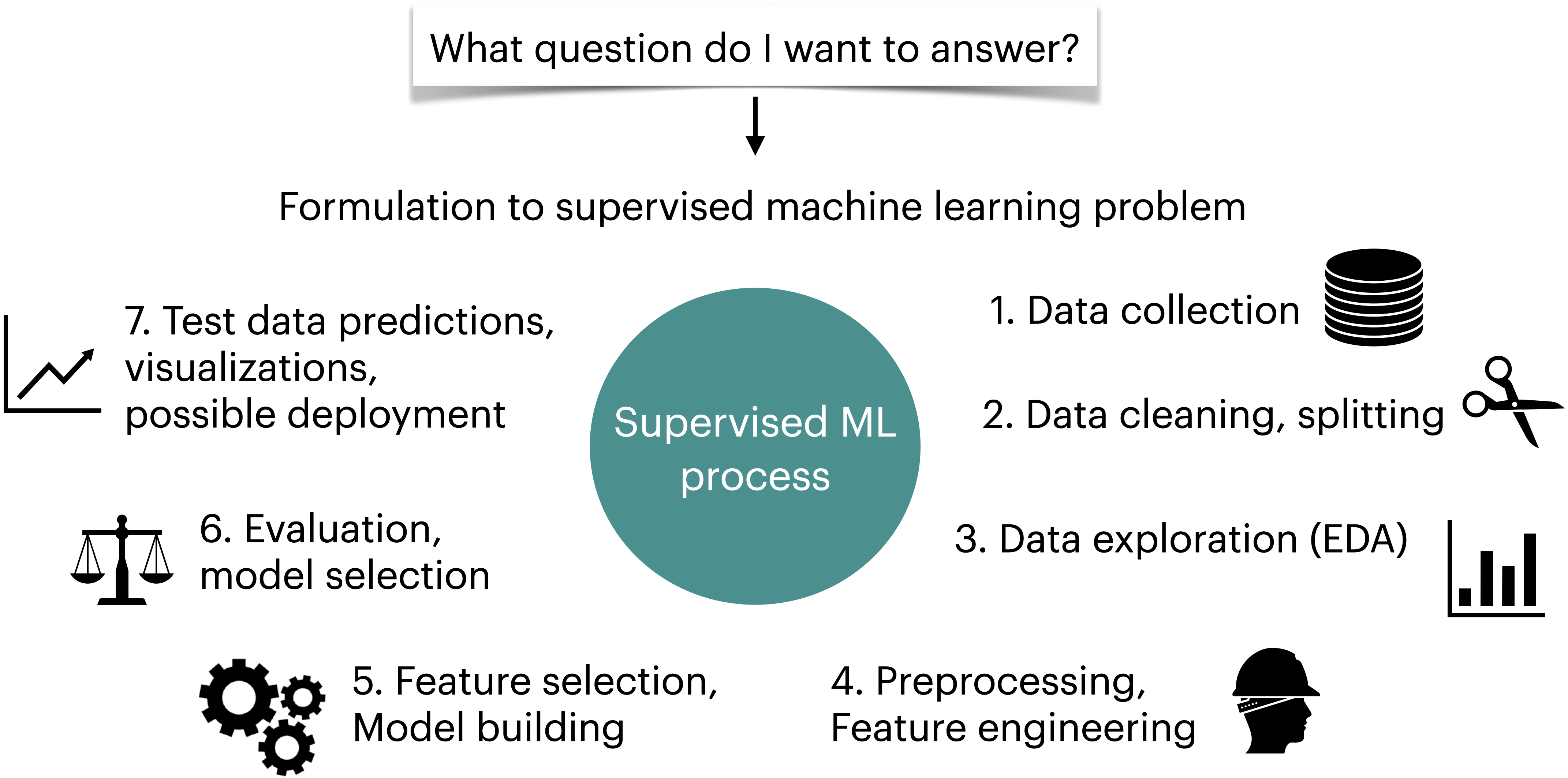
Machine learning workflow

• Here is a typical workflow of a supervised machine learning systems.

• So far, we have talked about data splitting, preprocessing, some EDA, model selection with hyperparameter optimization, and interpretation in the context of linear models.

• In the next few lectures, we will talk about evaluation metrics and model selection in terms of evaluation metrics, feature engineering, feature selection, and model transparency and interpretation.

Evaluation metrics for binary classification: Motivation

Dataset for demonstration

• Let’s classify fraudulent and non-fraudulent transactions using Kaggle’s Credit Card Fraud Detection data set.

cc_df = pd.read_csv("data/creditcard.csv", encoding="latin-1")
train_df, test_df = train_test_split(cc_df, test_size=0.3, random_state=111)
train_df.head()

	Time	V1	V2	V3	V4	V5	V6	V7	V8	V9	...	V21	V22	V23	V24	V25	V26	V27	V28	Amount	Class
64454	51150.0	-3.538816	3.481893	-1.827130	-0.573050	2.644106	-0.340988	2.102135	-2.939006	2.578654	...	0.530978	-0.860677	-0.201810	-1.719747	0.729143	-0.547993	-0.023636	-0.454966	1.00	0
37906	39163.0	-0.363913	0.853399	1.648195	1.118934	0.100882	0.423852	0.472790	-0.972440	0.033833	...	0.687055	-0.094586	0.121531	0.146830	-0.944092	-0.558564	-0.186814	-0.257103	18.49	0
79378	57994.0	1.193021	-0.136714	0.622612	0.780864	-0.823511	-0.706444	-0.206073	-0.016918	0.781531	...	-0.310405	-0.842028	0.085477	0.366005	0.254443	0.290002	-0.036764	0.015039	23.74	0
245686	152859.0	1.604032	-0.808208	-1.594982	0.200475	0.502985	0.832370	-0.034071	0.234040	0.550616	...	0.519029	1.429217	-0.139322	-1.293663	0.037785	0.061206	0.005387	-0.057296	156.52	0
60943	49575.0	-2.669614	-2.734385	0.662450	-0.059077	3.346850	-2.549682	-1.430571	-0.118450	0.469383	...	-0.228329	-0.370643	-0.211544	-0.300837	-1.174590	0.573818	0.388023	0.161782	57.50	0

5 rows × 31 columns

train_df.shape

(199364, 31)

• Good size dataset

• For confidentially reasons, it only provides transformed features with PCA, which is a popular dimensionality reduction technique.

EDA

train_df.info()

<class 'pandas.core.frame.DataFrame'>
Index: 199364 entries, 64454 to 129900
Data columns (total 31 columns):
 #   Column  Non-Null Count   Dtype  
---  ------  --------------   -----  
 0   Time    199364 non-null  float64
 1   V1      199364 non-null  float64
 2   V2      199364 non-null  float64
 3   V3      199364 non-null  float64
 4   V4      199364 non-null  float64
 5   V5      199364 non-null  float64
 6   V6      199364 non-null  float64
 7   V7      199364 non-null  float64
 8   V8      199364 non-null  float64
 9   V9      199364 non-null  float64
 10  V10     199364 non-null  float64
 11  V11     199364 non-null  float64
 12  V12     199364 non-null  float64
 13  V13     199364 non-null  float64
 14  V14     199364 non-null  float64
 15  V15     199364 non-null  float64
 16  V16     199364 non-null  float64
 17  V17     199364 non-null  float64
 18  V18     199364 non-null  float64
 19  V19     199364 non-null  float64
 20  V20     199364 non-null  float64
 21  V21     199364 non-null  float64
 22  V22     199364 non-null  float64
 23  V23     199364 non-null  float64
 24  V24     199364 non-null  float64
 25  V25     199364 non-null  float64
 26  V26     199364 non-null  float64
 27  V27     199364 non-null  float64
 28  V28     199364 non-null  float64
 29  Amount  199364 non-null  float64
 30  Class   199364 non-null  int64  
dtypes: float64(30), int64(1)
memory usage: 48.7 MB

train_df.describe(include="all")

	Time	V1	V2	V3	V4	V5	V6	V7	V8	V9	...	V21	V22	V23	V24	V25	V26	V27	V28	Amount	Class
count	199364.000000	199364.000000	199364.000000	199364.000000	199364.000000	199364.000000	199364.000000	199364.000000	199364.000000	199364.000000	...	199364.000000	199364.000000	199364.000000	199364.000000	199364.000000	199364.000000	199364.000000	199364.000000	199364.000000	199364.000000
mean	94888.815669	0.000492	-0.000726	0.000927	0.000630	0.000036	0.000011	-0.001286	-0.002889	-0.000891	...	0.001205	0.000155	-0.000198	0.000113	0.000235	0.000312	-0.000366	0.000227	88.164679	0.001700
std	47491.435489	1.959870	1.645519	1.505335	1.413958	1.361718	1.327188	1.210001	1.214852	1.096927	...	0.748510	0.726634	0.628139	0.605060	0.520857	0.481960	0.401541	0.333139	238.925768	0.041201
min	0.000000	-56.407510	-72.715728	-31.813586	-5.683171	-42.147898	-26.160506	-43.557242	-73.216718	-13.320155	...	-34.830382	-8.887017	-44.807735	-2.824849	-10.295397	-2.241620	-22.565679	-11.710896	0.000000	0.000000
25%	54240.000000	-0.918124	-0.600193	-0.892476	-0.847178	-0.691241	-0.768512	-0.553979	-0.209746	-0.642965	...	-0.227836	-0.541795	-0.162330	-0.354604	-0.317761	-0.326730	-0.070929	-0.052819	5.640000	0.000000
50%	84772.500000	0.018854	0.065463	0.179080	-0.019531	-0.056703	-0.275290	0.040497	0.022039	-0.052607	...	-0.029146	0.007666	-0.011678	0.041031	0.016587	-0.052790	0.001239	0.011234	22.000000	0.000000
75%	139349.250000	1.315630	0.803617	1.028023	0.744201	0.610407	0.399827	0.570449	0.327408	0.597326	...	0.186899	0.529210	0.146809	0.439209	0.351366	0.242169	0.090453	0.078052	77.150000	0.000000
max	172792.000000	2.451888	22.057729	9.382558	16.491217	34.801666	23.917837	44.054461	19.587773	15.594995	...	27.202839	10.503090	22.083545	4.022866	6.070850	3.517346	12.152401	33.847808	11898.090000	1.000000

8 rows × 31 columns

• We do not have categorical features. All features are numeric.

• We have to be careful about the Time and Amount features.

• We could scale Amount.

• Do we want to scale time?

  • In this lecture, we’ll just drop the Time feature.

  • We’ll learn about time series briefly later in the course.

Let’s separate X and y for train and test splits.

X_train_big, y_train_big = train_df.drop(columns=["Class", "Time"]), train_df["Class"]
X_test, y_test = test_df.drop(columns=["Class", "Time"]), test_df["Class"]

• It’s easier to demonstrate evaluation metrics using an explicit validation set instead of using cross-validation.

• So let’s create a validation set.

• Our data is large enough so it shouldn’t be a problem.

X_train, X_valid, y_train, y_valid = train_test_split(
    X_train_big, y_train_big, test_size=0.3, random_state=123
)

Baseline

dummy = DummyClassifier()
pd.DataFrame(cross_validate(dummy, X_train, y_train, return_train_score=True)).mean()

fit_time       0.007850
score_time     0.001011
test_score     0.998302
train_score    0.998302
dtype: float64

Observations

• DummyClassifier is getting 0.998 cross-validation accuracy!!

• Should we be happy with this accuracy and deploy this DummyClassifier model for fraud detection?

What’s the class distribution?

train_df["Class"].value_counts(normalize=True)

Class
0    0.9983
1    0.0017
Name: proportion, dtype: float64

• We have class imbalance.

• We have MANY non-fraud transactions and only a handful of fraud transactions.

• So in the training set, most_frequent strategy is labeling 199,025 (99.83%) instances correctly and only 339 (0.17%) instances incorrectly.

• Is this what we want?

• The “fraud” class is the important class that we want to spot.

Let’s scale the features and try LogisticRegression.

pipe = make_pipeline(StandardScaler(), LogisticRegression())
pd.DataFrame(cross_validate(pipe, X_train, y_train, return_train_score=True)).mean()

fit_time       0.230603
score_time     0.003676
test_score     0.999176
train_score    0.999235
dtype: float64

• We are getting a slightly better score with logistic regression.

• What score should be considered an acceptable score here?

• Are we actually spotting any “fraud” transactions?

• .score by default returns accuracy which is $\(\frac{\text{correct predictions}}{\text{total examples}}\)$

• Is accuracy a good metric here?

• Is there anything more informative than accuracy that we can use here?

Let’s dig a little deeper.

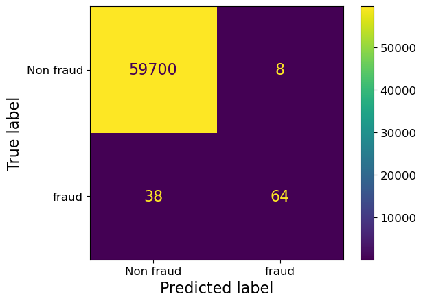
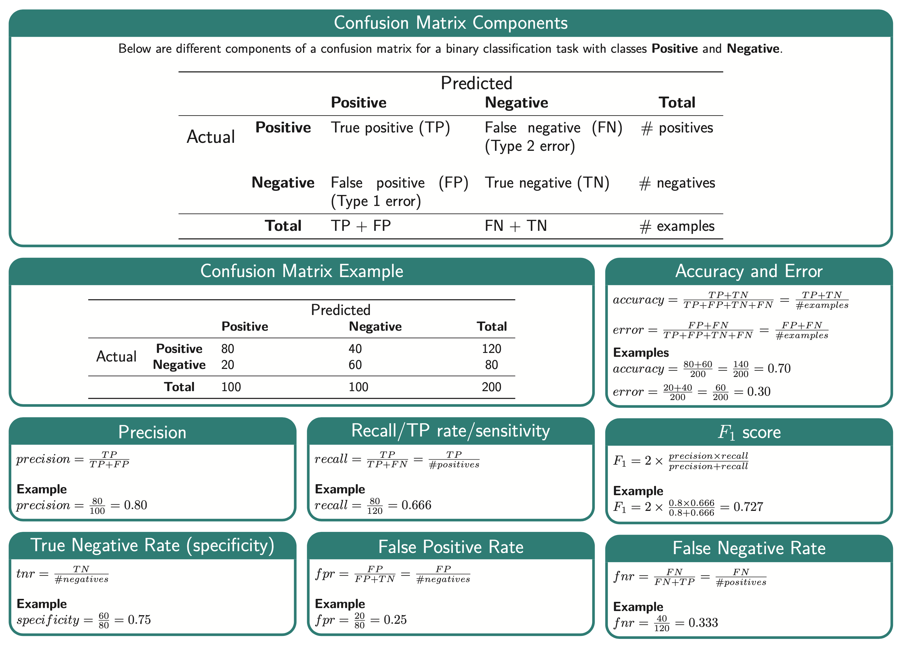
Confusion matrix

One way to get a better understanding of the errors is by looking at

• false positives (type I errors), where the model incorrectly spots examples as fraud

• false negatives (type II errors), where it’s missing to spot fraud examples

from sklearn.metrics import ConfusionMatrixDisplay  # Recommended method in sklearn 1.0

pipe.fit(X_train, y_train)
cm = ConfusionMatrixDisplay.from_estimator(
    pipe, X_valid, y_valid, values_format="d", display_labels=["Non fraud", "fraud"]
)

from sklearn.metrics import confusion_matrix

predictions = pipe.predict(X_valid)
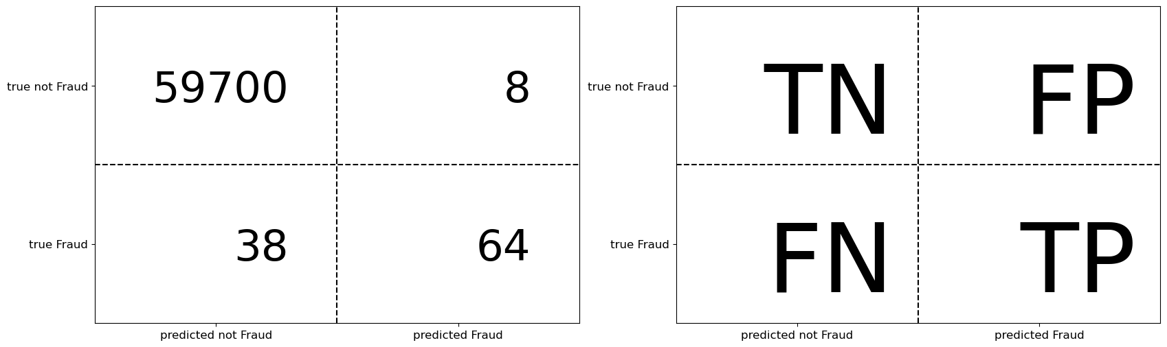
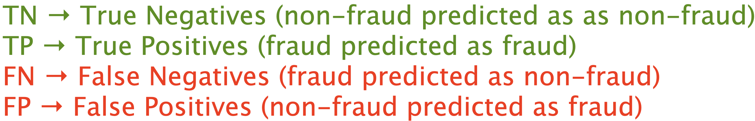
TN, FP, FN, TP = confusion_matrix(y_valid, predictions).ravel()
plot_confusion_matrix_example(TN, FP, FN, TP)

• Perfect prediction has all values down the diagonal

• Off diagonal entries can often tell us about what is being mis-predicted

What is “positive” and “negative”?

• Two kinds of binary classification problems

  • Distinguishing between two classes

  • Spotting a class (spot fraud transaction, spot spam, spot disease)

• In case of spotting problems, the thing that we are interested in spotting is considered “positive”.

• Above we wanted to spot fraudulent transactions and so they are “positive”.

You can get a numpy array of confusion matrix as follows:

from sklearn.metrics import confusion_matrix

predictions = pipe.predict(X_valid)
TN, FP, FN, TP = confusion_matrix(y_valid, predictions).ravel()
print("Confusion matrix for fraud data set")
print(cm.confusion_matrix)

Confusion matrix for fraud data set
[[59700     8]
 [   38    64]]

Confusion matrix with cross-validation

• You can also calculate confusion matrix with cross-validation using the cross_val_predict method.

• But then you cannot plot it in a nice format.

from sklearn.model_selection import cross_val_predict

confusion_matrix(y_train, cross_val_predict(pipe, X_train, y_train))

array([[139296,     21],
       [    94,    143]])

Precision, recall, f1 score

• We have been using .score to assess our models, which returns accuracy by default.

• Accuracy is misleading when we have class imbalance.

• We need other metrics to assess our models.

• We’ll discuss three commonly used metrics which are based on confusion matrix:

  • recall

  • precision

  • f1 score

• Note that these metrics will only help us assess our model.

• Later we’ll talk about a few ways to address class imbalance problem.

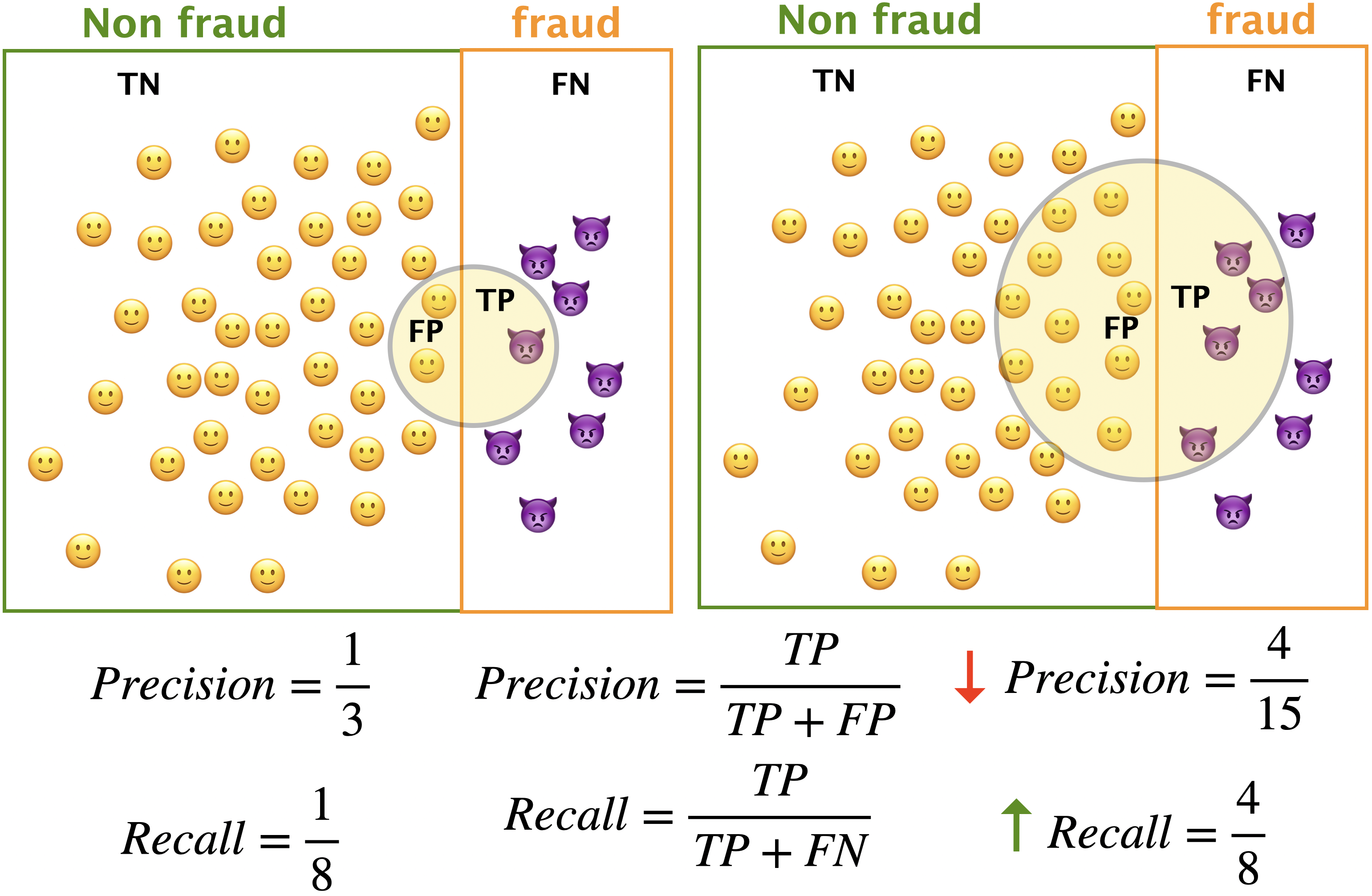
Precision and recall: toy example

• Imagine that your model has identified everything outside the circle as non-fraud and everything inside the circle as fraud.

from sklearn.metrics import confusion_matrix

pipe_lr = make_pipeline(StandardScaler(), LogisticRegression())
pipe_lr.fit(X_train, y_train)
predictions = pipe_lr.predict(X_valid)
TN, FP, FN, TP = confusion_matrix(y_valid, predictions).ravel()
print(cm.confusion_matrix)

[[59700     8]
 [   38    64]]

Precision

Among the positive examples you identified, how many were actually positive?

\[ precision = \frac{TP}{TP+FP}\]

cm = ConfusionMatrixDisplay.from_estimator(
    pipe, X_valid, y_valid, values_format="d", display_labels=["Non fraud", "fraud"]
);

print("TP = %0.4f, FP = %0.4f" % (TP, FP))
precision = TP / (TP + FP)
print("Precision: %0.4f" % (precision))

TP = 64.0000, FP = 8.0000
Precision: 0.8889

Recall

Among all positive examples, how many did you identify correctly? $\( recall = \frac{TP}{TP+FN} = \frac{TP}{\#positives} \)$

• Also called as sensitivity, coverage, true positive rate (TPR)

ConfusionMatrixDisplay.from_estimator(
    pipe, X_valid, y_valid, values_format="d", display_labels=["Non fraud", "fraud"]
);

print("TP = %0.4f, FN = %0.4f" % (TP, FN))
recall = TP / (TP + FN)
print("Recall: %0.4f" % (recall))

TP = 64.0000, FN = 38.0000
Recall: 0.6275

F1-score

• F1-score combines precision and recall to give one score, which could be used in hyperparameter optimization, for instance.

• F1-score is a harmonic mean of precision and recall.

\[ f1 = 2 \times \frac{ precision \times recall}{precision + recall}\]

print("precision: %0.4f" % (precision))
print("recall: %0.4f" % (recall))
f1_score = (2 * precision * recall) / (precision + recall)
print("f1: %0.4f" % (f1_score))

precision: 0.8889
recall: 0.6275
f1: 0.7356

Let’s look at all metrics at once on our dataset.

## Calculate evaluation metrics by ourselves
data = {
    "calculation": [],
    "accuracy": [],
    "error": [],
    "precision": [],
    "recall": [],
    "f1 score": [],
}
data["calculation"].append("manual")
data["accuracy"].append((TP + TN) / (TN + FP + FN + TP))
data["error"].append((FP + FN) / (TN + FP + FN + TP))
data["precision"].append(precision)  # TP / (TP + FP)
data["recall"].append(recall)  # TP / (TP + FN)
data["f1 score"].append(f1_score)  # (2 * precision * recall) / (precision + recall)
df = pd.DataFrame(data)
df

	calculation	accuracy	error	precision	recall	f1 score
0	manual	0.999231	0.000769	0.888889	0.627451	0.735632

• scikit-learn has functions for these metrics.

from sklearn.metrics import accuracy_score, f1_score, precision_score, recall_score

data["accuracy"].append(accuracy_score(y_valid, pipe_lr.predict(X_valid)))
data["error"].append(1 - accuracy_score(y_valid, pipe_lr.predict(X_valid)))
data["precision"].append(
    precision_score(y_valid, pipe_lr.predict(X_valid), zero_division=1)
)
data["recall"].append(recall_score(y_valid, pipe_lr.predict(X_valid)))
data["f1 score"].append(f1_score(y_valid, pipe_lr.predict(X_valid)))
data["calculation"].append("sklearn")
df = pd.DataFrame(data)
df.set_index(["calculation"])

	accuracy	error	precision	recall	f1 score
calculation
manual	0.999231	0.000769	0.888889	0.627451	0.735632
sklearn	0.999231	0.000769	0.888889	0.627451	0.735632

The scores match.

Classification report

• There is a convenient function called classification_report in sklearn which gives this info.

pipe_lr.classes_

array([0, 1])

from sklearn.metrics import classification_report

print(
    classification_report(
        y_valid, pipe_lr.predict(X_valid), target_names=["non-fraud", "fraud"]
    )
)

              precision    recall  f1-score   support

   non-fraud       1.00      1.00      1.00     59708
       fraud       0.89      0.63      0.74       102

    accuracy                           1.00     59810
   macro avg       0.94      0.81      0.87     59810
weighted avg       1.00      1.00      1.00     59810

(Optional) Macro average and weighted average

Macro average

• Gives equal importance to all classes and average over all classes.

• For instance, in the example above, recall for non-fraud is 1.0 and fraud is 0.63, and so macro average is 0.81.

• More relevant in case of multi-class problems.

Weighted average

• Weighted by the number of samples in each class.

• Divide by the total number of samples.

Which one is relevant when depends upon whether you think each class should have the same weight or each sample should have the same weight.

Toy example

from sklearn.metrics import classification_report
y_true_toy = [0, 1, 0, 1, 0]
y_pred_toy = [0, 0, 0, 1, 0]
target_names_toy = ['class 0', 'class 1']
print(classification_report(y_true_toy, y_pred_toy, target_names=target_names_toy))

              precision    recall  f1-score   support

     class 0       0.75      1.00      0.86         3
     class 1       1.00      0.50      0.67         2

    accuracy                           0.80         5
   macro avg       0.88      0.75      0.76         5
weighted avg       0.85      0.80      0.78         5

• weighted average is weighted by the proportion of examples in a particular class. So for the toy example above:

• weighted_average precision: 3/5 * 0.75 + 2/5 * 1.00 = 0.85

• weighted_average recall: 3/5 * 1.00 + 2/5 * 0.5 = 0.80

• weighted_average f1-score: 3/5 * 0.86 + 2/5 * 0.67 = 0.78

• macro average gives equal weight to both classes. So for the toy example above:

• macro average precision: 0.5 * 0.75 + 0.5 * 1.00 =0. 875

• macro average recall: 0.5 * 1.00 + 0.5 * 0.5 =0. 75

• macro average f1-score: 0.5 * 0.75 + 0.5 * 1.00 =0.765

Interim summary

• Accuracy is misleading when you have class imbalance.

• A confusion matrix provides a way to break down errors made by our model.

• We looked at three metrics based on confusion matrix:

  • precision, recall, f1-score.

• Note that what you consider “positive” (fraud in our case) is important when calculating precision, recall, and f1-score.

• If you flip what is considered positive or negative, we’ll end up with different TP, FP, TN, FN, and hence different precision, recall, and f1-scores.

Evalution metrics overview

There is a lot of terminology here.

Cross validation with different metrics

• We can pass different evaluation metrics with scoring argument of cross_validate.

scoring = [
    "accuracy",
    "f1",
    "recall",
    "precision",
]  # scoring can be a string, a list, or a dictionary
pipe = make_pipeline(StandardScaler(), LogisticRegression())
scores = cross_validate(
    pipe, X_train_big, y_train_big, return_train_score=True, scoring=scoring
)
pd.DataFrame(scores)

	fit_time	score_time	test_accuracy	train_accuracy	test_f1	train_f1	test_recall	train_recall	test_precision	train_precision
0	0.354016	0.022270	0.999097	0.999360	0.694915	0.782979	0.602941	0.678967	0.820000	0.924623
1	0.305161	0.020853	0.999223	0.999317	0.739496	0.766595	0.647059	0.660517	0.862745	0.913265
2	0.303150	0.021214	0.999273	0.999216	0.743363	0.726477	0.617647	0.612546	0.933333	0.892473
3	0.309229	0.021295	0.999172	0.999254	0.697248	0.742981	0.558824	0.634686	0.926829	0.895833
4	0.301052	0.020986	0.999147	0.999216	0.696429	0.728850	0.582090	0.617647	0.866667	0.888889

• You can also create your own scoring function and pass it to cross_validate.

(Optional) Evaluation metrics for multi-class classification

Let’s examine precision, recall, and f1-score of different classes in the HappyDB corpus.

df = pd.read_csv("data/cleaned_hm.csv", index_col=0)
sample_df = df.dropna()
sample_df.head()
sample_df = sample_df.rename(
    columns={"cleaned_hm": "moment", "ground_truth_category": "target"}
)
sample_df.head()

	wid	reflection_period	original_hm	moment	modified	num_sentence	target	predicted_category
hmid
27676	206	24h	We had a serious talk with some friends of ours who have been flaky lately. They understood and we had a good evening hanging out.	We had a serious talk with some friends of ours who have been flaky lately. They understood and we had a good evening hanging out.	True	2	bonding	bonding
27678	45	24h	I meditated last night.	I meditated last night.	True	1	leisure	leisure
27697	498	24h	My grandmother start to walk from the bed after a long time.	My grandmother start to walk from the bed after a long time.	True	1	affection	affection
27705	5732	24h	I picked my daughter up from the airport and we have a fun and good conversation on the way home.	I picked my daughter up from the airport and we have a fun and good conversation on the way home.	True	1	bonding	affection
27715	2272	24h	when i received flowers from my best friend	when i received flowers from my best friend	True	1	bonding	bonding

train_df, test_df = train_test_split(sample_df, test_size=0.3, random_state=123)
X_train_happy, y_train_happy = train_df["moment"], train_df["target"]
X_test_happy, y_test_happy = test_df["moment"], test_df["target"]

from sklearn.feature_extraction.text import CountVectorizer

pipe_lr = make_pipeline(
    CountVectorizer(stop_words="english"), LogisticRegression(max_iter=2000)
)

pipe_lr.fit(X_train_happy, y_train_happy)
pred = pipe_lr.predict(X_test_happy)

ConfusionMatrixDisplay.from_estimator(
    pipe_lr, X_test_happy, y_test_happy, xticks_rotation="vertical"
);

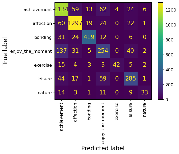
print(classification_report(y_test_happy, pred))

                  precision    recall  f1-score   support

     achievement       0.79      0.87      0.83      1302
       affection       0.90      0.91      0.91      1423
         bonding       0.91      0.85      0.88       492
enjoy_the_moment       0.60      0.54      0.57       469
        exercise       0.91      0.57      0.70        74
         leisure       0.73      0.70      0.71       407
          nature       0.73      0.46      0.57        71

        accuracy                           0.82      4238
       macro avg       0.80      0.70      0.74      4238
    weighted avg       0.82      0.82      0.81      4238

• Seems like there is a lot of variation in the scores for different classes. The model is performing pretty well on affection class but not that well on enjoy_the_moment and nature classes.

• If each class is equally important for you, pick macro avg as your evaluation metric.

• If each example is equally important, pick weighted avg as your metric.

❓❓ Questions for you

iClicker Exercise 1.1

iClicker cloud join link: https://join.iclicker.com/SNBF

Select all of the following statements which are TRUE.

• (A) In medical diagnosis, false positives are more damaging than false negatives (assume “positive” means the person has a disease, “negative” means they don’t).

• (B) In spam classification, false positives are more damaging than false negatives (assume “positive” means the email is spam, “negative” means they it’s not).

• (C) If method A gets a higher accuracy than method B, that means its precision is also higher.

• (D) If method A gets a higher accuracy than method B, that means its recall is also higher.

V’s answers: (B)

Method A - higher accuracy but lower precision

Negative	Positive
90	5
5	0

Method B - lower accuracy but higher precision

Negative	Positive
80	15
0	5

Precision-recall curve

• Confusion matrix provides a detailed break down of the errors made by the model.

• But when creating a confusion matrix, we are using “hard” predictions.

• Most classifiers in scikit-learn provide predict_proba method (or decision_function) which provides degree of certainty about predictions by the classifier.

• Can we explore the degree of uncertainty to understand and improve the model performance?

Let’s revisit the classification report on our fraud detection example.

pipe_lr = make_pipeline(StandardScaler(), LogisticRegression())
pipe_lr.fit(X_train, y_train);

y_pred = pipe_lr.predict(X_valid)
print(classification_report(y_valid, y_pred, target_names=["non-fraud", "fraud"]))

              precision    recall  f1-score   support

   non-fraud       1.00      1.00      1.00     59708
       fraud       0.89      0.63      0.74       102

    accuracy                           1.00     59810
   macro avg       0.94      0.81      0.87     59810
weighted avg       1.00      1.00      1.00     59810

By default, predictions use the threshold of 0.5. If predict_proba > 0.5, predict “fraud” else predict “non-fraud”.

y_pred = pipe_lr.predict_proba(X_valid)[:, 1] > 0.50
print(classification_report(y_valid, y_pred, target_names=["non-fraud", "fraud"]))

              precision    recall  f1-score   support

   non-fraud       1.00      1.00      1.00     59708
       fraud       0.89      0.63      0.74       102

    accuracy                           1.00     59810
   macro avg       0.94      0.81      0.87     59810
weighted avg       1.00      1.00      1.00     59810

• Suppose for your business it is more costly to miss fraudulent transactions and suppose you want to achieve a recall of at least 75% for the “fraud” class.

• One way to do this is by changing the threshold of predict_proba.

  • predict returns 1 when predict_proba’s probabilities are above 0.5 for the “fraud” class.

Key idea: what if we threshold the probability at a smaller value so that we identify more examples as “fraud” examples?

Let’s lower the threshold to 0.1. In other words, predict the examples as “fraud” if predict_proba > 0.1.

y_pred_lower_threshold = pipe_lr.predict_proba(X_valid)[:, 1] > 0.1

print(classification_report(y_valid, y_pred_lower_threshold))

              precision    recall  f1-score   support

           0       1.00      1.00      1.00     59708
           1       0.77      0.76      0.77       102

    accuracy                           1.00     59810
   macro avg       0.89      0.88      0.88     59810
weighted avg       1.00      1.00      1.00     59810

Operating point

• Now our recall for “fraud” class is >= 0.75.

• Setting a requirement on a classifier (e.g., recall of >= 0.75) is called setting the operating point.

• It’s usually driven by business goals and is useful to make performance guarantees to customers.

Precision/Recall tradeoff

• But there is a trade-off between precision and recall.

• If you identify more things as “fraud”, recall is going to increase but there are likely to be more false positives.

Let’s sweep through different thresholds.

thresholds = np.arange(0.0, 1.0, 0.1)
thresholds

array([0. , 0.1, 0.2, 0.3, 0.4, 0.5, 0.6, 0.7, 0.8, 0.9])

You need to install panel package in order to run the code below locally. See the documentation here.

conda install -c pyviz panel

import panel as pn
from panel import widgets
from panel.interact import interact

pn.extension()

def f(threshold):
    preds = pipe_lr.predict_proba(X_valid)[:, 1] > threshold
    precision = np.round(precision_score(y_valid, preds), 4)
    recall = np.round(recall_score(y_valid, preds), 4)
    d = {'threshold':np.round(threshold, 4), 'Precision': precision, 'recall': recall}
    return (d)

interact(f, threshold=widgets.FloatSlider(start=0.0, end=0.99, step=0.05, value=0.5)).embed(max_opts=20)

Decreasing the threshold

• Decreasing the threshold means a lower bar for predicting fraud.

  • You are willing to risk more false positives in exchange of more true positives.

  • Recall would either stay the same or go up and precision is likely to go down

  • Occasionally, precision may increase if all the new examples after decreasing the threshold are TPs.

Increasing the threshold

• Increasing the threshold means a higher bar for predicting fraud.

  • Recall would go down or stay the same but precision is likely to go up

  • Occasionally, precision may go down if TP decrease but FP do not decrease.

Precision-recall curve

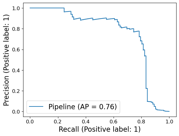
Often, when developing a model, it’s not always clear what the operating point will be and to understand the model better, it’s informative to look at all possible thresholds and corresponding trade-offs of precision and recall in a plot.

from sklearn.metrics import precision_recall_curve

precision, recall, thresholds = precision_recall_curve(
    y_valid, pipe_lr.predict_proba(X_valid)[:, 1]
)
plt.plot(precision, recall, label="logistic regression: PR curve")
plt.xlabel("Precision")
plt.ylabel("Recall")
plt.plot(
    precision_score(y_valid, pipe_lr.predict(X_valid)),
    recall_score(y_valid, pipe_lr.predict(X_valid)),
    "or",
    markersize=10,
    label="threshold 0.5",
)
plt.legend(loc="best");

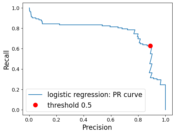
• Each point in the curve corresponds to a possible threshold of the predict_proba output.

• We can achieve a recall of 0.8 at a precision of 0.4.

• The red dot marks the point corresponding to the threshold 0.5.

• The top-right would be a perfect classifier (precision = recall = 1).

• The threshold is not shown here, but it’s going from 0 (upper-left) to 1 (lower right).

• At a threshold of 0 (upper left), we are classifying everything as “fraud”.

• Raising the threshold increases the precision but at the expense of lowering the recall.

• At the extreme right, where the threshold is 1, we get into the situation where all the examples classified as “fraud” are actually “fraud”; we have no false positives.

• Here we have a high precision but lower recall.

• Usually the goal is to keep recall high as precision goes up.

AP score

• Often it’s useful to have one number summarizing the PR plot (e.g., in hyperparameter optimization)

• One way to do this is by computing the area under the PR curve.

• This is called average precision (AP score)

• AP score has a value between 0 (worst) and 1 (best).

from sklearn.metrics import average_precision_score

ap_lr = average_precision_score(y_valid, pipe_lr.predict_proba(X_valid)[:, 1])
print("Average precision of logistic regression: {:.3f}".format(ap_lr))

Average precision of logistic regression: 0.757

You can also use the following handy function of sklearn to get the PR curve and the corresponding AP score.

from sklearn.metrics import PrecisionRecallDisplay

PrecisionRecallDisplay.from_estimator(pipe_lr, X_valid, y_valid);

AP vs. F1-score

It is very important to note this distinction:

• F1 score is for a given threshold and measures the quality of predict.

• AP score is a summary across thresholds and measures the quality of predict_proba.

Important

Remember to pick the desired threshold based on the results on the validation set and not on the test set.

A few comments on PR curve

• Different classifiers might work well in different parts of the curve, i.e., at different operating points.

• We can compare PR curves of different classifiers to understand these differences.

• Let’s create PR curves for SVC and Logistic Regression.

pipe_svc = make_pipeline(StandardScaler(), SVC())

pipe_svc.fit(X_train, y_train)

pipe_lr = make_pipeline(StandardScaler(), LogisticRegression(max_iter=1000))
pipe_lr.fit(X_train, y_train)

Pipeline(steps=[('standardscaler', StandardScaler()),
                ('logisticregression', LogisticRegression(max_iter=1000))])

In a Jupyter environment, please rerun this cell to show the HTML representation or trust the notebook.
On GitHub, the HTML representation is unable to render, please try loading this page with nbviewer.org.

How to get precision and recall for different thresholds?

• Use the function precision_recall_curve

precision_lr, recall_lr, thresholds_lr = precision_recall_curve(
    y_valid, pipe_lr.predict_proba(X_valid)[:, 1]
)

(Optional) Some more details

• How are the thresholds and the precision and recall at the default threshold are calculated?

How many thresholds?

• It uses n_thresholds where n_thresholds is the number of unique predict_proba scores in our dataset.

len(np.unique(pipe_lr.predict_proba(X_valid)[:, 1]))

59049

• For each threshold, precision and recall are calculated.

• The last precision and recall values are 1. and 0. respectively and do not have a corresponding threshold.

thresholds_lr.shape, precision_lr.shape, recall_lr.shape

((59049,), (59050,), (59050,))

precision_lr, recall_lr, thresholds_lr = precision_recall_curve(
    y_valid, pipe_lr.predict_proba(X_valid)[:, 1]
)
precision_svc, recall_svc, thresholds_svc = precision_recall_curve(
    y_valid, pipe_svc.decision_function(X_valid)
)

For logistic regression, what’s the index of the threshold that is closest to the default threshold of 0.5?

• We are subtracting 0.5 from the thresholds so that

  • the numbers close to 0 become -0.5

  • the numbers close to 1 become 0.5

  • the numbers close to 0.5 become 0

• After this transformation, we are interested in the threshold index where the number is close to 0. So we take absolute values and argmin.

close_default_lr = np.argmin(np.abs(thresholds_lr - 0.5))

SVC doesn’t have predict_proba. Instead it has something called decision_function. The index of the threshold that is closest to 0 of decision function is the default threshold in SVC.

close_zero_svm = np.argmin(np.abs(thresholds_svc))

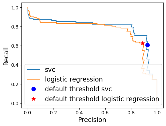
PR curves for logistic regression and SVC

plt.plot(precision_svc, recall_svc, label="svc")
plt.plot(precision_lr, recall_lr, label="logistic regression")
plt.plot(
    precision_svc[close_zero_svm],
    recall_svc[close_zero_svm],
    "o",
    markersize=10,
    label="default threshold svc",
    c="b",
)
plt.plot(
    precision_lr[close_default_lr],
    recall_lr[close_default_lr],
    "*",
    markersize=10,
    label="default threshold logistic regression",
    c="r",
)

plt.xlabel("Precision")
plt.ylabel("Recall")
plt.legend(loc="best");

svc_preds = pipe_svc.predict(X_valid)
lr_preds = pipe_lr.predict(X_valid)

print("f1_score of logistic regression: {:.3f}".format(f1_score(y_valid, lr_preds)))
print("f1_score of svc: {:.3f}".format(f1_score(y_valid, svc_preds)))

f1_score of logistic regression: 0.736
f1_score of svc: 0.726

ap_lr = average_precision_score(y_valid, pipe_lr.predict_proba(X_valid)[:, 1])
ap_svc = average_precision_score(y_valid, pipe_svc.decision_function(X_valid))

print("Average precision of logistic regression: {:.3f}".format(ap_lr))
print("Average precision of SVC: {:.3f}".format(ap_svc))

Average precision of logistic regression: 0.757
Average precision of SVC: 0.790

• Comparing the precision-recall curves provide us a detail insight compared to f1 score.

• For example, F1 scores for SVC and logistic regressions are pretty similar. In fact, f1 score of logistic regression is a tiny bit better.

• But when we look at the PR curve, we see that SVC is doing better than logistic regression for most of the other thresholds.

Receiver Operating Characteristic (ROC) curve

• Another commonly used tool to analyze the behavior of classifiers at different thresholds.

• Similar to PR curve, it considers all possible thresholds for a given classifier given by predict_proba but instead of precision and recall it plots false positive rate (FPR) and true positive rate (TPR or recall). $\( TPR = \frac{TP}{TP + FN}\)$

\[ FPR = \frac{FP}{FP + TN}\]

• TPR \(\rightarrow\) Fraction of true positives out of all positive examples.

• FPR \(\rightarrow\) Fraction of false positives out of all negative examples.

from sklearn.metrics import roc_curve

fpr, tpr, thresholds = roc_curve(y_valid, pipe_lr.predict_proba(X_valid)[:, 1])
plt.plot(fpr, tpr, label="ROC Curve")
plt.xlabel("FPR")
plt.ylabel("TPR (recall)")

default_threshold = np.argmin(np.abs(thresholds - 0.5))

plt.plot(
    fpr[default_threshold],
    tpr[default_threshold],
    "or",
    markersize=10,
    label="threshold 0.5",
)
plt.legend(loc="best");

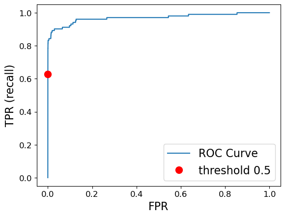
• Different points on the ROC curve represent different classification thresholds. The curve starts at (0,0) and ends at (1, 1).

  • (0, 0) represents the threshold that classifies everything as the negative class

  • (1, 1) represents the threshold that classifies everything as the positive class

• The ideal curve is close to the top left

  • Ideally, you want a classifier with high recall while keeping low false positive rate.

• The red dot corresponds to the threshold of 0.5, which is used by predict.

• We see that compared to the default threshold, we can achieve a better recall of around 0.8 without increasing FPR.

Let’s compare ROC curve of different classifiers.

fpr_lr, tpr_lr, thresholds_lr = roc_curve(y_valid, pipe_lr.predict_proba(X_valid)[:, 1])

fpr_svc, tpr_svc, thresholds_svc = roc_curve(
    y_valid, pipe_svc.decision_function(X_valid)
)

close_default_lr = np.argmin(np.abs(thresholds_lr - 0.5))
close_zero_svm = np.argmin(np.abs(thresholds_svc))

plt.plot(fpr_svc, tpr_svc, label="svc")
plt.plot(fpr_lr, tpr_lr, label="logistic regression")
plt.plot(
    fpr_svc[close_zero_svm],
    tpr_svc[close_zero_svm],
    "o",
    markersize=10,
    label="default threshold svc",
    c="b",
)
plt.plot(
    fpr_lr[close_default_lr],
    tpr_lr[close_default_lr],
    "*",
    markersize=10,
    label="default threshold logistic regression",
    c="r",
)

plt.xlabel("False positive rate")
plt.ylabel("True positive rate (Recall)")
plt.legend(loc="best");

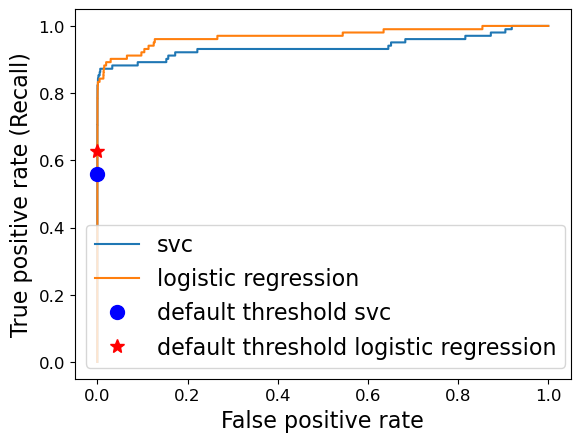
Area under the curve (AUC)

• AUC provides a single meaningful number for the model performance.

from sklearn.metrics import roc_auc_score

roc_lr = roc_auc_score(y_valid, pipe_lr.predict_proba(X_valid)[:, 1])
roc_svc = roc_auc_score(y_valid, pipe_svc.decision_function(X_valid))
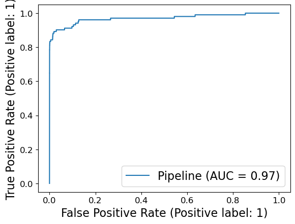
print("AUC for LR: {:.3f}".format(roc_lr))
print("AUC for SVC: {:.3f}".format(roc_svc))

AUC for LR: 0.970
AUC for SVC: 0.938

• AUC of 0.5 means random chance.

• AUC can be interpreted as evaluating the ranking of positive examples.

• What’s the probability that a randomly picked positive point has a higher score according to the classifier than a randomly picked point from the negative class.

• AUC of 1.0 means all positive points have a higher score than all negative points.

Important

For classification problems with imbalanced classes, using AP score or AUC is often much more meaningful than using accuracy.

Similar to PrecisionRecallCurveDisplay, there is a RocCurveDisplay function in sklearn.

from sklearn.metrics import RocCurveDisplay

RocCurveDisplay.from_estimator(pipe_lr, X_valid, y_valid);

Let’s look at all the scores at once

scoring = ["accuracy", "f1", "recall", "precision", "roc_auc", "average_precision"]
pipe = make_pipeline(StandardScaler(), LogisticRegression())
scores = cross_validate(pipe, X_train_big, y_train_big, scoring=scoring)
pd.DataFrame(scores).mean()

fit_time                  0.355054
score_time                0.044189
test_accuracy             0.999182
test_f1                   0.714290
test_recall               0.601712
test_precision            0.881915
test_roc_auc              0.967228
test_average_precision    0.744074
dtype: float64

See also

Check out these visualization on ROC and AUC.

See also

Check out how to plot ROC with cross-validation here.

Dealing with class imbalance [video]

Class imbalance in training sets

• This typically refers to having many more examples of one class than another in one’s training set.

• Real world data is often imbalanced.

  • Our Credit Card Fraud dataset is imbalanced.

  • Ad clicking data is usually drastically imbalanced. (Only around ~0.01% ads are clicked.)

  • Spam classification datasets are also usually imbalanced.

Addressing class imbalance

A very important question to ask yourself: “Why do I have a class imbalance?”

• Is it because one class is much more rare than the other?

  • If it’s just because one is more rare than the other, you need to ask whether you care about one type of error more than the other.

• Is it because of my data collection methods?

  • If it’s the data collection, then that means your test and training data come from different distributions!

In some cases, it may be fine to just ignore the class imbalance.

Which type of error is more important?

• False positives (FPs) and false negatives (FNs) have quite different real-world consequences.

• In PR curve and ROC curve, we saw how changing the prediction threshold can change FPs and FNs.

• We can then pick the threshold that’s appropriate for our problem.

• Example: if we want high recall, we may use a lower threshold (e.g., a threshold of 0.1). We’ll then catch more fraudulent transactions.

pipe_lr = make_pipeline(StandardScaler(), LogisticRegression())
pipe_lr.fit(X_train, y_train)
y_pred = pipe_lr.predict(X_valid)
print(classification_report(y_valid, y_pred, target_names=["non-fraud", "fraud"]))

              precision    recall  f1-score   support

   non-fraud       1.00      1.00      1.00     59708
       fraud       0.89      0.63      0.74       102

    accuracy                           1.00     59810
   macro avg       0.94      0.81      0.87     59810
weighted avg       1.00      1.00      1.00     59810

y_pred = pipe_lr.predict_proba(X_valid)[:, 1] > 0.10
print(classification_report(y_valid, y_pred, target_names=["non-fraud", "fraud"]))

              precision    recall  f1-score   support

   non-fraud       1.00      1.00      1.00     59708
       fraud       0.77      0.76      0.77       102

    accuracy                           1.00     59810
   macro avg       0.89      0.88      0.88     59810
weighted avg       1.00      1.00      1.00     59810

Handling imbalance

Can we change the model itself rather than changing the threshold so that it takes into account the errors that are important to us?

There are two common approaches for this:

• Changing the data (optional) (not covered in this course)

  • Undersampling

  • Oversampling

    • Random oversampling

    • SMOTE

• Changing the training procedure

  • class_weight

Changing the training procedure

• All sklearn classifiers have a parameter called class_weight.

• This allows you to specify that one class is more important than another.

• For example, maybe a false negative is 10x more problematic than a false positive.

Example: class_weight parameter of sklearn LogisticRegression

class sklearn.linear_model.LogisticRegression(penalty=’l2’, dual=False, tol=0.0001, C=1.0, fit_intercept=True, intercept_scaling=1, class_weight=None, random_state=None, solver=’lbfgs’, max_iter=100, multi_class=’auto’, verbose=0, warm_start=False, n_jobs=None, l1_ratio=None)

class_weight: dict or ‘balanced’, default=None

Weights associated with classes in the form {class_label: weight}. If not given, all classes are supposed to have weight one.

import IPython
url = "https://scikit-learn.org/stable/modules/generated/sklearn.linear_model.LogisticRegression.html"
IPython.display.IFrame(width=1000, height=650, src=url)

# plot_confusion_matrix(
#     pipe_lr,
#     X_valid,
#     y_valid,
#     display_labels=["Non fraud", "fraud"],
#     values_format="d",
#     cmap=plt.cm.Blues,
# );

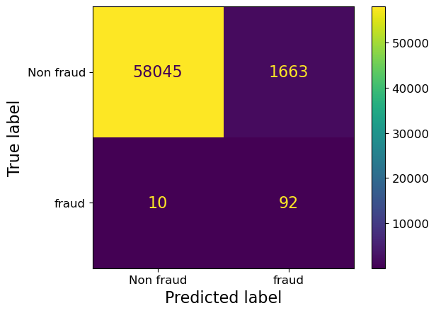
ConfusionMatrixDisplay.from_estimator(
    pipe_lr, X_valid, y_valid, display_labels=["Non fraud", "fraud"], values_format="d"
);

pipe_lr.named_steps["logisticregression"].classes_

array([0, 1])

Let’s set “fraud” class a weight of 10.

pipe_lr_weight = make_pipeline(
    StandardScaler(), LogisticRegression(max_iter=500, class_weight={0: 1, 1: 10})
)
pipe_lr_weight.fit(X_train, y_train)
ConfusionMatrixDisplay.from_estimator(
    pipe_lr_weight,
    X_valid,
    y_valid,
    display_labels=["Non fraud", "fraud"],
    values_format="d",
);

• Notice we’ve reduced false negatives and predicted more Fraud this time.

• This was equivalent to saying give 10x more “importance” to fraud class.

• Note that as a consequence we are also increasing false positives.

class_weight="balanced"

• A useful setting is class_weight="balanced".

• This sets the weights so that the classes are “equal”.

class_weight: dict, ‘balanced’ or None If ‘balanced’, class weights will be given by n_samples / (n_classes * np.bincount(y)). If a dictionary is given, keys are classes and values are corresponding class weights. If None is given, the class weights will be uniform.

sklearn.utils.class_weight.compute_class_weight(class_weight, classes, y)

pipe_lr_balanced = make_pipeline(
    StandardScaler(), LogisticRegression(max_iter=500, class_weight="balanced")
)
pipe_lr_balanced.fit(X_train, y_train)
ConfusionMatrixDisplay.from_estimator(
    pipe_lr_balanced,
    X_valid,
    y_valid,
    display_labels=["Non fraud", "fraud"],
    values_format="d",
);

We have reduced false negatives but we have many more false positives now …

Are we doing better with class_weight="balanced"?

comp_dict = {}
pipe_lr = make_pipeline(StandardScaler(), LogisticRegression(max_iter=500))
scoring = ["accuracy", "f1", "recall", "precision", "roc_auc", "average_precision"]
orig_scores = cross_validate(pipe_lr, X_train_big, y_train_big, scoring=scoring)

pipe_lr_balanced = make_pipeline(
    StandardScaler(), LogisticRegression(max_iter=500, class_weight="balanced")
)
scoring = ["accuracy", "f1", "recall", "precision", "roc_auc", "average_precision"]
bal_scores = cross_validate(pipe_lr_balanced, X_train_big, y_train_big, scoring=scoring)
comp_dict = {
    "Original": pd.DataFrame(orig_scores).mean().tolist(),
    "class_weight='balanced'": pd.DataFrame(bal_scores).mean().tolist(),
}

pd.DataFrame(comp_dict, index=bal_scores.keys())

	Original	class_weight='balanced'
fit_time	0.351211	0.354338
score_time	0.045152	0.044722
test_accuracy	0.999182	0.973210
test_f1	0.714290	0.101817
test_recall	0.601712	0.891001
test_precision	0.881915	0.054009
test_roc_auc	0.967228	0.970505
test_average_precision	0.744074	0.730368

• Recall is much better but precision has dropped a lot; we have many false positives.

• You could also optimize class_weight using hyperparameter optimization for your specific problem.

• Changing the class weight will generally reduce accuracy.

• The original model was trying to maximize accuracy.

• Now you’re telling it to do something different.

• But that can be fine, accuracy isn’t the only metric that matters.

Stratified Splits

• A similar idea of “balancing” classes can be applied to data splits.

• We have the same option in train_test_split with the stratify argument.

• By default it splits the data so that if we have 10% negative examples in total, then each split will have 10% negative examples.

• If you are carrying out cross validation using cross_validate, by default it uses StratifiedKFold. From the documentation:

This cross-validation object is a variation of KFold that returns stratified folds. The folds are made by preserving the percentage of samples for each class.

• In other words, if we have 10% negative examples in total, then each fold will have 10% negative examples.

Is stratifying a good idea?

• Well, it’s no longer a random sample, which is probably theoretically bad, but not that big of a deal.

• If you have many examples, it shouldn’t matter as much.

• It can be especially useful in multi-class, say if you have one class with very few cases.

• In general, these are difficult questions.

(Optional) Changing the data

• Undersampling

• Oversampling

  • Random oversampling

  • SMOTE

We cannot use sklearn pipelines because of some API related problems. But there is something called imbalance learn, which is an extension of the scikit-learn API that allows us to resample. It’s already in our course environment. If you don’t have the course environment installed, you can install it in your environment with this command:

conda install -c conda-forge imbalanced-learn

Undersampling

import imblearn
from imblearn.pipeline import make_pipeline as make_imb_pipeline
from imblearn.under_sampling import RandomUnderSampler

rus = RandomUnderSampler()
X_train_subsample, y_train_subsample = rus.fit_resample(X_train, y_train)
print(X_train.shape)
print(X_train_subsample.shape)
print(np.bincount(y_train_subsample))

(139554, 29)
(474, 29)
[237 237]

from collections import Counter

from imblearn.under_sampling import RandomUnderSampler
from sklearn.datasets import make_classification

X, y = make_classification(
    n_classes=2,
    class_sep=2,
    weights=[0.1, 0.9],
    n_informative=3,
    n_redundant=1,
    flip_y=0,
    n_features=20,
    n_clusters_per_class=1,
    n_samples=1000,
    random_state=10,
)
print("Original dataset shape %s" % Counter(y))
rus = RandomUnderSampler(random_state=42)
X_res, y_res = rus.fit_resample(X, y)
print("Resampled dataset shape %s" % Counter(y_res))

Original dataset shape Counter({1: 900, 0: 100})
Resampled dataset shape Counter({0: 100, 1: 100})

undersample_pipe = make_imb_pipeline(
    RandomUnderSampler(), StandardScaler(), LogisticRegression()
)
scores = cross_validate(
    undersample_pipe, X_train, y_train, scoring=("roc_auc", "average_precision")
)
pd.DataFrame(scores).mean()

fit_time                  0.040014
score_time                0.016725
test_roc_auc              0.965142
test_average_precision    0.464847
dtype: float64

Oversampling

• Random oversampling with replacement

• SMOTE: Synthetic Minority Over-sampling Technique

from imblearn.over_sampling import RandomOverSampler

ros = RandomOverSampler()
X_train_oversample, y_train_oversample = ros.fit_resample(X_train, y_train)
print(X_train.shape)
print(X_train_oversample.shape)
print(np.bincount(y_train_oversample))

(139554, 29)
(278634, 29)
[139317 139317]

oversample_pipe = make_imb_pipeline(
    RandomOverSampler(), StandardScaler(), LogisticRegression(max_iter=1000)
)
scores = cross_validate(
    oversample_pipe, X_train, y_train, scoring=("roc_auc", "average_precision")
)
pd.DataFrame(scores).mean()

fit_time                  1.312607
score_time                0.015294
test_roc_auc              0.961708
test_average_precision    0.715192
dtype: float64

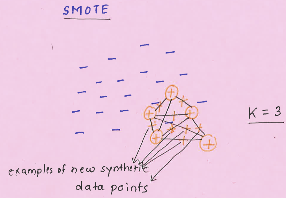
SMOTE: Synthetic Minority Over-sampling Technique

sklearn SMOTE

• Create “synthetic” examples rather than by over-sampling with replacement.

• Inspired by a technique of data augmentation that proved successful in handwritten character recognition.

• The minority class is over-sampled by taking each minority class sample and introducing synthetic examples along the line segments joining any/all of the \(k\) minority class nearest neighbors.

• \(k\) is chosen depending upon the amount of over-sampling required.

SMOTE idea

• Take the difference between the feature vector (sample) under consideration and its nearest neighbor.

• Multiply this difference by a random number between 0 and 1, and add it to the feature vector under consideration.

• This causes the selection of a random point along the line segment between two specific features.

• This approach effectively forces the decision region of the minority class to become more general.

Using SMOTE

• You need to imbalanced-learn

class imblearn.over_sampling.SMOTE(sampling_strategy=’auto’, random_state=None, k_neighbors=5, m_neighbors=’deprecated’, out_step=’deprecated’, kind=’deprecated’, svm_estimator=’deprecated’, n_jobs=1, ratio=None)

Class to perform over-sampling using SMOTE.

This object is an implementation of SMOTE - Synthetic Minority Over-sampling Technique as presented in this paper.

from imblearn.over_sampling import SMOTE

smote_pipe = make_imb_pipeline(
    SMOTE(), StandardScaler(), LogisticRegression(max_iter=1000)
)
scores = cross_validate(
    smote_pipe, X_train, y_train, cv=10, scoring=("roc_auc", "average_precision")
)
pd.DataFrame(scores).mean()

fit_time                  1.324045
score_time                0.014373
test_roc_auc              0.962920
test_average_precision    0.732802
dtype: float64

• We got higher average precision score with SMOTE in this case.

• These are rather simple approaches to tackle class imbalance.

• If you have a problem such as fraud detection problem where you want to spot rare events, you can think of this problem as anomaly detection problem and use algorithms such as isolation forests.

• If you are interested in this area, it might be worth checking out this book on this topic. (I’ve not read it.)

  • Imbalanced Learning: Foundations, Algorithms, and Applications

  • It’s available via UBC library.

ML fairness activity (~5 mins)

AI/ML systems can give the illusion of objectivity as they are derived from seemingly unbiased data & algorithm. However, human are inherently biased and AI/ML systems, if not carefully evaluated, can even further amplify the existing inequities and systemic bias in our society.

How do we make sure our AI/ML systems are fair? Which metrics can we use to quantify ‘fairness’ in AI/ML systems?

Let’s examine this on the adult census data set.

census_df = pd.read_csv("data/adult.csv")
census_df.shape

(32561, 15)

train_df, test_df = train_test_split(census_df, test_size=0.4, random_state=42)

train_df

	age	workclass	fnlwgt	education	education.num	marital.status	occupation	relationship	race	sex	capital.gain	capital.loss	hours.per.week	native.country	income
25823	36	Private	245521	7th-8th	4	Married-civ-spouse	Farming-fishing	Husband	White	Male	0	0	35	Mexico	<=50K
10274	26	Private	134287	Assoc-voc	11	Never-married	Sales	Own-child	White	Female	0	0	35	United-States	<=50K
27652	25	Local-gov	109526	HS-grad	9	Married-civ-spouse	Craft-repair	Husband	White	Male	0	0	38	United-States	<=50K
13941	23	Private	131275	HS-grad	9	Never-married	Craft-repair	Own-child	Amer-Indian-Eskimo	Male	0	0	40	United-States	<=50K
31384	27	Private	193122	HS-grad	9	Married-civ-spouse	Machine-op-inspct	Husband	White	Male	0	0	40	United-States	<=50K
...	...	...	...	...	...	...	...	...	...	...	...	...	...	...	...
29802	25	Private	410240	HS-grad	9	Never-married	Craft-repair	Own-child	White	Male	0	0	40	United-States	<=50K
5390	51	Private	146767	Assoc-voc	11	Married-civ-spouse	Prof-specialty	Husband	White	Male	0	0	40	United-States	>50K
860	55	Federal-gov	238192	HS-grad	9	Married-civ-spouse	Tech-support	Husband	White	Male	0	1887	40	United-States	>50K
15795	41	Private	154076	Some-college	10	Married-civ-spouse	Adm-clerical	Husband	White	Male	0	0	50	United-States	>50K
23654	22	Private	162667	HS-grad	9	Never-married	Handlers-cleaners	Own-child	White	Male	0	0	50	Portugal	<=50K

19536 rows × 15 columns

train_df_nan = train_df.replace("?", np.nan)
test_df_nan = test_df.replace("?", np.nan)
train_df_nan.shape

(19536, 15)

# Let's identify numeric and categorical features

numeric_features = [
    "age",
    "capital.gain",
    "capital.loss",
    "hours.per.week",
]

categorical_features = [
    "workclass",
    "marital.status",
    "occupation",
    "relationship",
    "race",
    "native.country",
]

ordinal_features = ["education"]
binary_features = [
    "sex"
]  # Not binary in general but in this particular dataset it seems to have only two possible values
drop_features = ["education.num", "fnlwgt"]
target = "income"

train_df["education"].unique()

array(['7th-8th', 'Assoc-voc', 'HS-grad', 'Bachelors', 'Some-college',
       '10th', '11th', 'Prof-school', '12th', '5th-6th', 'Masters',
       'Assoc-acdm', '9th', 'Doctorate', '1st-4th', 'Preschool'],
      dtype=object)

education_levels = [
    "Preschool",
    "1st-4th",
    "5th-6th",
    "7th-8th",
    "9th",
    "10th",
    "11th",
    "12th",
    "HS-grad",
    "Prof-school",
    "Assoc-voc",
    "Assoc-acdm",
    "Some-college",
    "Bachelors",
    "Masters",
    "Doctorate",
]

assert set(education_levels) == set(train_df["education"].unique())

X_train = train_df_nan.drop(columns=[target])
y_train = train_df_nan[target]

X_test = test_df_nan.drop(columns=[target])
y_test = test_df_nan[target]

from sklearn.compose import ColumnTransformer, make_column_transformer
from sklearn.impute import SimpleImputer
from sklearn.preprocessing import OneHotEncoder, OrdinalEncoder, StandardScaler

numeric_transformer = make_pipeline(StandardScaler())

ordinal_transformer = OrdinalEncoder(categories=[education_levels], dtype=int)

categorical_transformer = make_pipeline(
    SimpleImputer(strategy="constant", fill_value="missing"),
    OneHotEncoder(handle_unknown="ignore", sparse_output=False),
)

binary_transformer = make_pipeline(
    SimpleImputer(strategy="constant", fill_value="missing"),
    OneHotEncoder(drop="if_binary", dtype=int),
)

preprocessor = make_column_transformer(
    (numeric_transformer, numeric_features),
    (ordinal_transformer, ordinal_features),
    (binary_transformer, binary_features),
    (categorical_transformer, categorical_features),
    ("drop", drop_features),
)

y_train.value_counts()

income
<=50K    14841
>50K      4695
Name: count, dtype: int64

pipe_lr = make_pipeline(
    preprocessor, LogisticRegression(class_weight="balanced", max_iter=1000)
)

pipe_lr.fit(X_train, y_train);

ConfusionMatrixDisplay.from_estimator(pipe_lr, X_test, y_test);

Let’s examine confusion matrix separately for the two genders we have in the data.

X_train_enc = preprocessor.fit_transform(X_train)
preprocessor.named_transformers_["pipeline-2"]["onehotencoder"].get_feature_names_out()

array(['x0_Male'], dtype=object)

X_test.head()

	age	workclass	fnlwgt	education	education.num	marital.status	occupation	relationship	race	sex	capital.gain	capital.loss	hours.per.week	native.country
14160	29	Private	280618	Some-college	10	Married-civ-spouse	Handlers-cleaners	Husband	White	Male	0	0	40	United-States
27048	19	Private	439779	Some-college	10	Never-married	Sales	Own-child	White	Male	0	0	15	United-States
28868	28	Private	204734	Some-college	10	Married-civ-spouse	Tech-support	Wife	White	Female	0	0	40	United-States
5667	35	Private	107991	11th	7	Never-married	Sales	Not-in-family	White	Male	0	0	45	United-States
7827	20	Private	54152	Some-college	10	Never-married	Adm-clerical	Own-child	White	Female	0	0	30	NaN

X_female = X_test.query("sex=='Female'")  # X where sex is female
X_male = X_test.query("sex=='Male'")  # X where sex is male

y_female = y_test[X_female.index]  # y where sex is female
y_male = y_test[X_male.index]  # y where sex is male

Get predictions for X_female and y_male with pipe_lr

female_preds = pipe_lr.predict(X_female)
male_preds = pipe_lr.predict(X_male)

Let’s examine the accuracy and confusion matrix for female and male classes.

print(classification_report(y_female, female_preds))

              precision    recall  f1-score   support

       <=50K       0.96      0.94      0.95      3851
        >50K       0.57      0.66      0.61       463

    accuracy                           0.91      4314
   macro avg       0.76      0.80      0.78      4314
weighted avg       0.92      0.91      0.91      4314

print(classification_report(y_male, male_preds))

              precision    recall  f1-score   support

       <=50K       0.91      0.72      0.80      6028
        >50K       0.57      0.85      0.68      2683

    accuracy                           0.76      8711
   macro avg       0.74      0.78      0.74      8711
weighted avg       0.81      0.76      0.77      8711

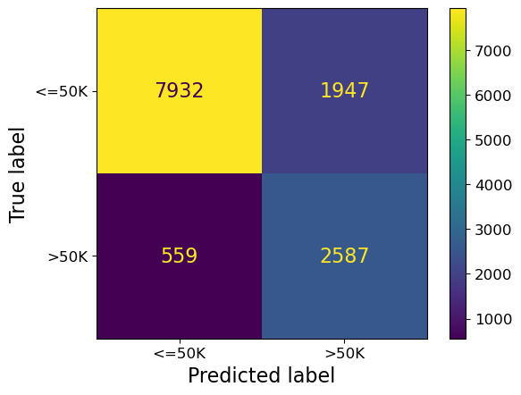
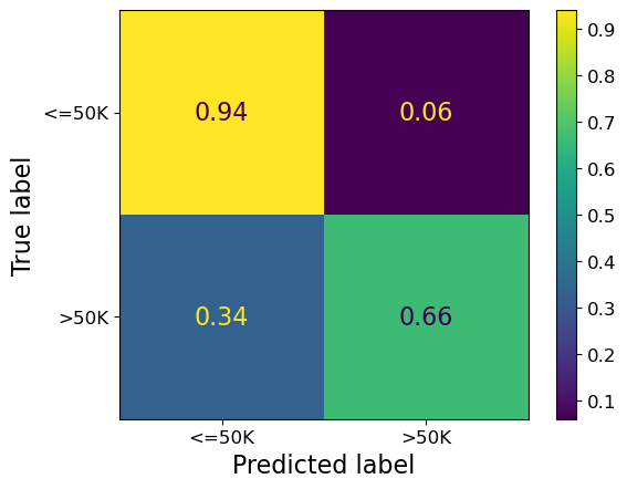
fig, axes = plt.subplots(1, 2, figsize=(15, 5))

# Plot the female confusion matrix
female_cm = ConfusionMatrixDisplay.from_estimator(pipe_lr, X_female, y_female, normalize="true");
axes[0].set_title('Confusion Matrix - Female');
female_cm.plot(ax=axes[0]);


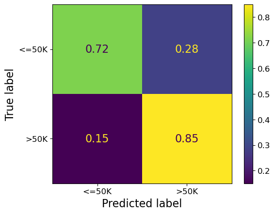
# Plot the male confusion matrix
male_cm = ConfusionMatrixDisplay.from_estimator(pipe_lr, X_male, y_male, normalize="true");
axes[1].set_title('Confusion Matrix - Male');
male_cm.plot(ax=axes[1]);

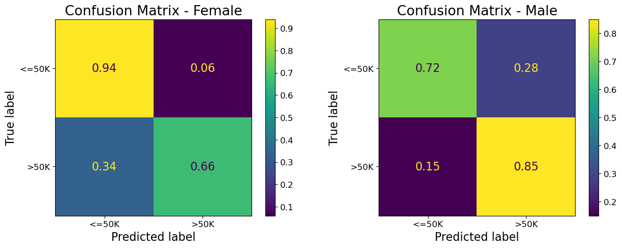
❓❓ Questions for group discussion

Let’s assume that a company is using this classifier for loan approval with a simple rule that if the income is >=50K, approve the loan else reject the loan.

In your group, discuss the questions below.

1. Which group has a higher accuracy?

2. Which group has a higher precision for class >50K? What about recall for class >50K?

3. Will both groups have more or less the same proportion of people with approved loans?

4. If a male and a female have both a certain level of income, will they have the same chance of getting the loan?

5. Banks want to avoid approving unqualified applications (false positives) because default loan could have detrimental effects for them. Compare the false positive rates for the two groups.

6. Overall, do you think this income classifier will fairly treat both groups? What will be the consequences of using this classifier in loan approval application?

Time permitting

1. Do you think the effect will still exist if the sex feature is removed from the model (but you still have it available separately to do the two confusion matrices)?

2. Are there any other groups in this dataset worth examining for biases?

What did we learn today?

• A number of possible ways to evaluate machine learning models

  • Choose the evaluation metric that makes most sense in your context or which is most common in your discipline

• Two kinds of binary classification problems

  • Distinguishing between two classes (e.g., dogs vs. cats)

  • Spotting a class (e.g., spot fraud transaction, spot spam)

• Precision, recall, f1-score are useful when dealing with spotting problems.

• The thing that we are interested in spotting is considered “positive”.

• Do you need to deal with class imbalance in the given problem?

• Methods to deal with class imbalance

  • Changing the training procedure

    • class_weight

  • Changing the data

    • undersampling, oversampling, SMOTE

• Do not blindly make decisions solely based on ML model predictions.

• Try to carefully analyze the errors made by the model on certain groups.

Relevant papers and resources

• The Relationship Between Precision-Recall and ROC Curves

• Article claiming that PR curve are better than ROC for imbalanced datasets

• Precision-Recall-Gain Curves: PR Analysis Done Right

• ROC animation

• Generalization in Adaptive Data Analysis and Holdout Reuse