Lecture 19: Time series

UBC 2023-24

Instructor: Varada Kolhatkar and Andrew Roth

The picture is created using DALL-E!

This illustration shows a cityscape with skyscrapers, each featuring digital billboards displaying time-series graphs. These graphs represent various types of data such as stock market trends, weather patterns, and population growth, set against the backdrop of a bustling city with people of diverse descents and genders. This setting should provide a compelling and relatable context for your introduction to time-series lecture.

Imports, announcements, LO

Imports

import matplotlib.pyplot as plt
import numpy as np
import pandas as pd
from sklearn.compose import ColumnTransformer, make_column_transformer
from sklearn.dummy import DummyClassifier
from sklearn.ensemble import RandomForestClassifier
from sklearn.impute import SimpleImputer
from sklearn.linear_model import LogisticRegression
from sklearn.model_selection import (
    TimeSeriesSplit,
    cross_val_score,
    cross_validate,
    train_test_split,
)
from sklearn.pipeline import Pipeline, make_pipeline
from sklearn.preprocessing import OneHotEncoder, OrdinalEncoder, StandardScaler

plt.rcParams["font.size"] = 12
from datetime import datetime

Announcements

• HW8 has been released. (Due next week Monday.)

• Thank you for filling out the midterm survey!

  • We’ll try to be more responsive on Piazza.

  • Our lectures are recorded. You can find the Panopto links for each section on Canvas.

Learning objectives

• Recognize when it is appropriate to use time series.

• Explain the pitfalls of train/test splitting with time series data.

• Appropriately split time series data, both train/test split and cross-validation.

• Perform time series feature engineering:

  • Encode time as various features in a tabular dataset

  • Create lag-based features

• Explain how can you forecast multiple time steps into the future.

• Explain the challenges of time series data with unequally spaced time points.

• At a high level, explain the concept of trend.

Motivation

• Time series is a collection of data points indexed in time order.

• Time series is everywhere:

  • Physical sciences (e.g., weather forecasting)

  • Economics, finance (e.g., stocks, market trends)

  • Engineering (e.g., energy consumption)

  • Social sciences

  • Sports analytics

Let’s start with a simple example from Introduction to Machine Learning with Python book.

In New York city there is a network of bike rental stations with a subscription system. The stations are all around the city. The anonymized data is available here.

We will focus on the task is predicting how many people will rent a bicycle from a particular station for a given time and day. We might be interested in knowing this so that we know whether there will be any bikes left at the station for a particular day and time.

import mglearn

citibike = mglearn.datasets.load_citibike()
citibike.head()

starttime
2015-08-01 00:00:00     3
2015-08-01 03:00:00     0
2015-08-01 06:00:00     9
2015-08-01 09:00:00    41
2015-08-01 12:00:00    39
Freq: 3H, Name: one, dtype: int64

• The only feature we have is the date time feature.

  • Example: 2015-08-01 00:00:00

• What’s the duration of the intervals?

  • The data is collected at regular intervals (every three hours)

• The target is the number of rentals in the next 3 hours.

  • Example: 3 rentals between 2015-08-01 00:00:00 and 2015-08-01 03:00:00

• We have a time-ordered sequence of data points.

• This type of data is distinctive because it is inherently sequential, with an intrinsic order based on time.

• The number of bikes available at a station at one point in time is often related to the number of bikes at earlier times.

• This is a time-series forecasting problem.

Let’s check the time duration of our data.

citibike.index.min()

Timestamp('2015-08-01 00:00:00')

citibike.index.max()

Timestamp('2015-08-31 21:00:00')

We have data for August 2015. Let’s visualize our data.

plt.figure(figsize=(8, 3))
xticks = pd.date_range(start=citibike.index.min(), end=citibike.index.max(), freq="D")
plt.xticks(xticks, xticks.strftime("%a %m-%d"), rotation=90, ha="left")
plt.plot(citibike, linewidth=1)
plt.xlabel("Date")
plt.ylabel("Rentals");
plt.title("Number of bike rentals over time for a selected bike station");

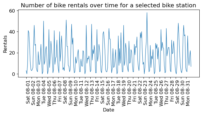
• We see the day and night pattern

• We see the weekend and weekday pattern

• Questions you might want to answer: How many people are likely to rent a bike at this station in the next three hours given everything we know about rentals in the past?

• We want to learn from the past and predict the future.

❓❓ Questions for you

• Can we use our usual supervised machine learning methodology to predict the number of people who will rent bicycles from a specific station at a given time and date?

• How can you adapt traditional machine learning methods for time series forecasting?

Train/test split for temporal data

• To evaluate the model’s ability to generalize, we will divide the data into training and testing subsets.

• What will happen if we split this data the usual way?

train_df, test_df = train_test_split(citibike, test_size=0.2, random_state=123)

test_df.head()

starttime
2015-08-26 12:00:00    30
2015-08-12 09:00:00    10
2015-08-19 03:00:00     2
2015-08-07 12:00:00    22
2015-08-03 09:00:00     9
Name: one, dtype: int64

plt.figure(figsize=(10, 3))
train_df_sort = train_df.sort_index()
test_df_sort = test_df.sort_index()

plt.plot(train_df_sort, "b", label="train")
plt.plot(test_df_sort, "r", label="test")
plt.xticks(rotation="vertical")
plt.legend();

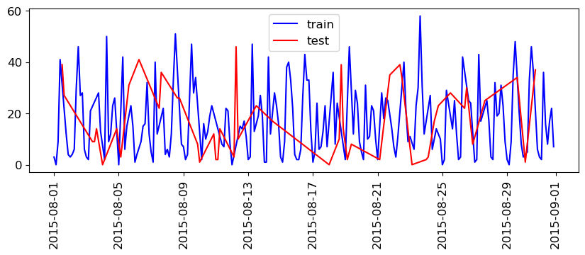
train_df.index.max()

Timestamp('2015-08-31 21:00:00')

test_df.index.min()

Timestamp('2015-08-01 12:00:00')

• So, we are training on data that came after our test data!

• If we want to forecast, we aren’t allowed to know what happened in the future!

• There may be cases where this is OK, e.g. if you aren’t trying to forecast and just want to understand your data (maybe you’re not even splitting).

• But, for our purposes, we want to avoid this.

We’ll split the data as follows:

• We have total 248 data points.

• We’ll use the fist 184 data points corresponding to the first 23 days as training data - And the remaining 64 data points corresponding to the remaining 8 days as test data.

citibike.shape

(248,)

n_train = 184
train_df = citibike[:184]
test_df = citibike[184:]

plt.figure(figsize=(10, 3))
train_df_sort = train_df.sort_index()
test_df_sort = test_df.sort_index()

plt.plot(train_df_sort, "b", label="train")
plt.plot(test_df_sort, "r", label="test")
plt.xticks(rotation="vertical")
plt.legend();

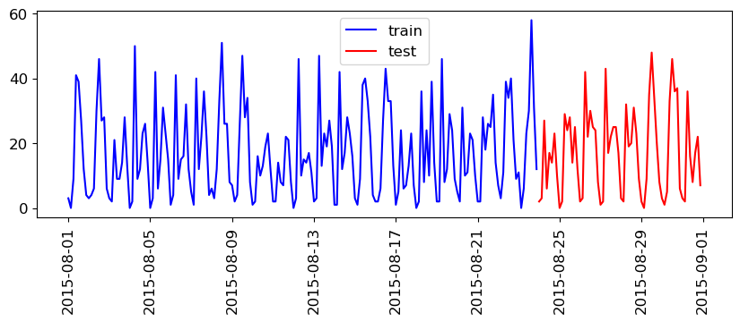
This split is looking reasonable now. We’ll train our model on the blue part and evaluate it on the red part.

train_df

starttime
2015-08-01 00:00:00     3
2015-08-01 03:00:00     0
2015-08-01 06:00:00     9
2015-08-01 09:00:00    41
2015-08-01 12:00:00    39
                       ..
2015-08-23 09:00:00    23
2015-08-23 12:00:00    30
2015-08-23 15:00:00    58
2015-08-23 18:00:00    31
2015-08-23 21:00:00    12
Freq: 3H, Name: one, Length: 184, dtype: int64

Feature engineering for date/time columns

❓❓ Questions for you

• What kind of features would you create from time series data to use in a model like a random forest or SVM?

POSIX time feature

• In this toy data, we just have a single feature: the date time feature.

• We need to encode this feature if we want to build machine learning models.

• A common way that dates are stored on computers is using POSIX time, which is the number of seconds since January 1970 00:00:00 (this is beginning of Unix time).

• Let’s start with encoding this feature as a single integer representing this POSIX time.

X = (
    citibike.index.astype("int64").values.reshape(-1, 1) // 10 ** 9
)  # convert to POSIX time by dividing by 10**9
y = citibike.values

Note

In pandas, datetime objects are typically represented as Timestamp objects, which internally store time as the number of nanoseconds (1 billionth of a second. 1 second = \(10^9\) nanoseconds) since the POSIX epoch (January 1, 1970, 00:00:00 UTC).

y_train = train_df.values
y_test = test_df.values
# convert to POSIX time by dividing by 10**9
X_train = train_df.index.astype("int64").values.reshape(-1, 1) // 10 ** 9
X_test = test_df.index.astype("int64").values.reshape(-1, 1) // 10 ** 9

X_train[:10]

array([[1438387200],
       [1438398000],
       [1438408800],
       [1438419600],
       [1438430400],
       [1438441200],
       [1438452000],
       [1438462800],
       [1438473600],
       [1438484400]])

y_train[:10]

array([ 3,  0,  9, 41, 39, 27, 12,  4,  3,  4])

• Our prediction task is a regression task.

• Let’s try random forest regression with just this feature.

• We’ll be trying out many different features. So we’ll be using the function below which

  • Splits the data

  • Trains the given regressor model on the training data

  • Shows train and test scores

  • Plots the predictions on the train and test data

# Code credit: Adapted from 
# https://learning.oreilly.com/library/view/introduction-to-machine/9781449369880/

def eval_on_features(features, target, regressor, n_train=184, sales_data=False, 
                     ylabel='Rentals', 
                     feat_names="Default", 
                     impute=True):
    """
    Evaluate a regression model on a given set of features and target.

    This function splits the data into training and test sets, fits the 
    regression model to the training data, and then evaluates and plots 
    the performance of the model on both the training and test datasets.

    Parameters:
    -----------
    features : array-like
        Input features for the model.
    target : array-like
        Target variable for the model.
    regressor : model object
        A regression model instance that follows the scikit-learn API.
    n_train : int, default=184
        The number of samples to be used in the training set.
    sales_data : bool, default=False
        Indicates if the data is sales data, which affects the plot ticks.
    ylabel : str, default='Rentals'
        The label for the y-axis in the plot.
    feat_names : str, default='Default'
        Names of the features used, for display in the plot title.
    impute : bool, default=True
        whether SimpleImputer needs to be applied or not

    Returns:
    --------
    None
        The function does not return any value. It prints the R^2 score
        and generates a plot.
    """

    # Split the features and target data into training and test sets
    X_train, X_test = features[:n_train], features[n_train:]
    y_train, y_test = target[:n_train], target[n_train:]

    if impute:
        simp = SimpleImputer()
        X_train = simp.fit_transform(X_train)
        X_test = simp.transform(X_test)
    
    # Fit the model on the training data
    regressor.fit(X_train, y_train)

    # Print R^2 scores for training and test datasets
    print("Train-set R^2: {:.2f}".format(regressor.score(X_train, y_train)))
    print("Test-set R^2: {:.2f}".format(regressor.score(X_test, y_test)))

    # Predict target variable for both training and test datasets
    y_pred_train = regressor.predict(X_train)
    y_pred = regressor.predict(X_test)

    # Plotting
    plt.figure(figsize=(10, 3))

    # If not sales data, adjust x-ticks for dates (assumes datetime format)
    if not sales_data: 
        plt.xticks(range(0, len(X), 8), xticks.strftime("%a %m-%d"), rotation=90, ha="left")

    # Plot training and test data, along with predictions
    plt.plot(range(n_train), y_train, label="train")
    plt.plot(range(n_train, len(y_test) + n_train), y_test, "-", label="test")
    plt.plot(range(n_train), y_pred_train, "--", label="prediction train")
    plt.plot(range(n_train, len(y_test) + n_train), y_pred, "--", label="prediction test")

    # Set plot title, labels, and legend
    title = regressor.__class__.__name__ + "\n Features= " + feat_names
    plt.title(title)
    plt.legend(loc=(1.01, 0))
    plt.xlabel("Date")
    plt.ylabel(ylabel)

Let’s try random forest regressor with our posix time feature.

from sklearn.ensemble import RandomForestRegressor

regressor = RandomForestRegressor(n_estimators=100, random_state=0)
eval_on_features(X, y, regressor, feat_names="POSIX time")

Train-set R^2: 0.85
Test-set R^2: -0.04

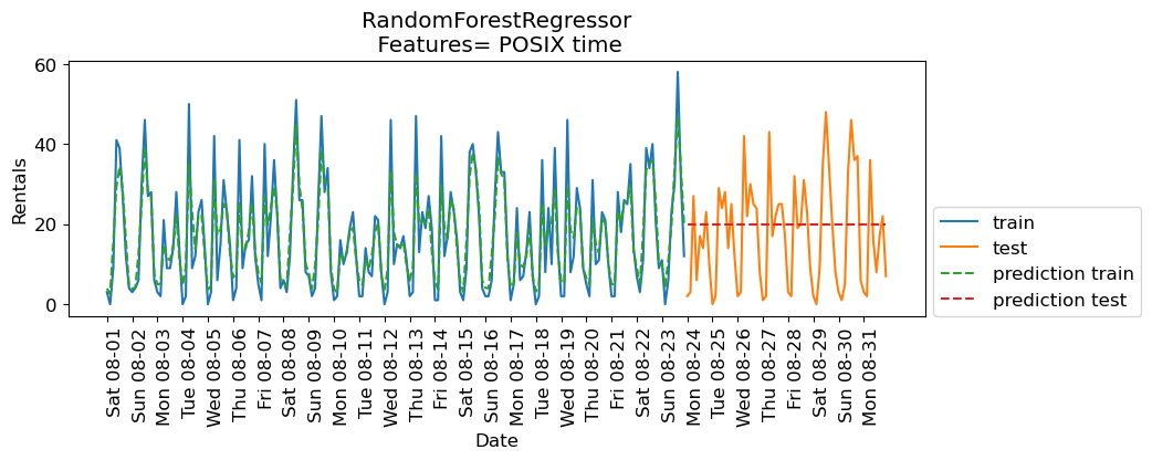
• The predictions on the training data and training score are pretty good

• But for the test data, a constant line is predicted …

• What’s going on?

• The model is based on only one feature: POSIX time feature.

• And the value of the POSIX time feature is outside the range of the feature values in the training set.

• Tree-based models cannot extrapolate to feature ranges outside the training data.

• The model predicted the target value of the closest point in the training set.

Can we come up with better features?

Extracting date and time information

• Note that our index is of this special type: DateTimeIndex. We can extract all kinds of interesting information from it.

citibike.index

DatetimeIndex(['2015-08-01 00:00:00', '2015-08-01 03:00:00',
               '2015-08-01 06:00:00', '2015-08-01 09:00:00',
               '2015-08-01 12:00:00', '2015-08-01 15:00:00',
               '2015-08-01 18:00:00', '2015-08-01 21:00:00',
               '2015-08-02 00:00:00', '2015-08-02 03:00:00',
               ...
               '2015-08-30 18:00:00', '2015-08-30 21:00:00',
               '2015-08-31 00:00:00', '2015-08-31 03:00:00',
               '2015-08-31 06:00:00', '2015-08-31 09:00:00',
               '2015-08-31 12:00:00', '2015-08-31 15:00:00',
               '2015-08-31 18:00:00', '2015-08-31 21:00:00'],
              dtype='datetime64[ns]', name='starttime', length=248, freq='3H')

citibike.index.month_name()

Index(['August', 'August', 'August', 'August', 'August', 'August', 'August',
       'August', 'August', 'August',
       ...
       'August', 'August', 'August', 'August', 'August', 'August', 'August',
       'August', 'August', 'August'],
      dtype='object', name='starttime', length=248)

citibike.index.dayofweek

Index([5, 5, 5, 5, 5, 5, 5, 5, 6, 6,
       ...
       6, 6, 0, 0, 0, 0, 0, 0, 0, 0],
      dtype='int32', name='starttime', length=248)

citibike.index.day_name()

Index(['Saturday', 'Saturday', 'Saturday', 'Saturday', 'Saturday', 'Saturday',
       'Saturday', 'Saturday', 'Sunday', 'Sunday',
       ...
       'Sunday', 'Sunday', 'Monday', 'Monday', 'Monday', 'Monday', 'Monday',
       'Monday', 'Monday', 'Monday'],
      dtype='object', name='starttime', length=248)

citibike.index.hour

Index([ 0,  3,  6,  9, 12, 15, 18, 21,  0,  3,
       ...
       18, 21,  0,  3,  6,  9, 12, 15, 18, 21],
      dtype='int32', name='starttime', length=248)

• We noted before that the time of the day and day of the week seem quite important.

• Let’s add these two features.

Let’s first add the time of the day.

X_hour = citibike.index.hour.values.reshape(-1, 1)
X_hour[:10]

array([[ 0],
       [ 3],
       [ 6],
       [ 9],
       [12],
       [15],
       [18],
       [21],
       [ 0],
       [ 3]], dtype=int32)

regressor = RandomForestRegressor(n_estimators=100, random_state=0)
eval_on_features(X_hour, y, regressor, feat_names = "Hour of the day")

Train-set R^2: 0.50
Test-set R^2: 0.60

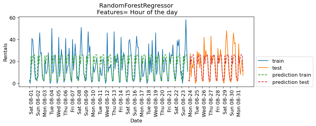
The scores are better when we add time of the day feature.

Now let’s add day of the week along with time of the day.

regressor = RandomForestRegressor(n_estimators=100, random_state=0)
X_hour_week = np.hstack(
    [
        citibike.index.dayofweek.values.reshape(-1, 1),
        citibike.index.hour.values.reshape(-1, 1),
    ]
)
eval_on_features(X_hour_week, y, regressor, feat_names = "hour of day + day of week")

Train-set R^2: 0.89
Test-set R^2: 0.84

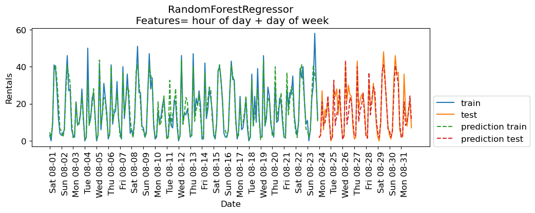
The results are much better. The time of the day and day of the week features are clearly helping.

• Do we need a complex model such as a random forest?

• Let’s try Ridge with these features.

from sklearn.linear_model import Ridge

lr = Ridge();
eval_on_features(X_hour_week, y, lr, feat_names = "hour of day + day of week")

Train-set R^2: 0.16
Test-set R^2: 0.13

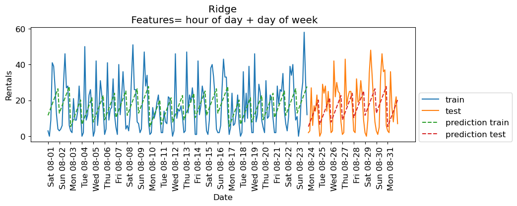
❓❓ Questions for you

• Why is Ridge performing poorly on the training data as well as test data?

Encoding time of day as a categorical feature

• Ridge is performing poorly because it’s not able to capture the periodic pattern.

• The reason is that we have encoded time of day using integers.

• A linear function can only learn a linear function of the time of day.

• What if we encode this feature as a categorical variable?

enc = OneHotEncoder()
X_hour_week_onehot = enc.fit_transform(X_hour_week).toarray()

X_hour_week_onehot
X_hour_week_onehot.shape

(248, 15)

hour = ["%02d:00" % i for i in range(0, 24, 3)]
day = ["Mon", "Tue", "Wed", "Thu", "Fri", "Sat", "Sun"]
features = day + hour

pd.DataFrame(X_hour_week_onehot, columns=features)

	Mon	Tue	Wed	Thu	Fri	Sat	Sun	00:00	03:00	06:00	09:00	12:00	15:00	18:00	21:00
0	0.0	0.0	0.0	0.0	0.0	1.0	0.0	1.0	0.0	0.0	0.0	0.0	0.0	0.0	0.0
1	0.0	0.0	0.0	0.0	0.0	1.0	0.0	0.0	1.0	0.0	0.0	0.0	0.0	0.0	0.0
2	0.0	0.0	0.0	0.0	0.0	1.0	0.0	0.0	0.0	1.0	0.0	0.0	0.0	0.0	0.0
3	0.0	0.0	0.0	0.0	0.0	1.0	0.0	0.0	0.0	0.0	1.0	0.0	0.0	0.0	0.0
4	0.0	0.0	0.0	0.0	0.0	1.0	0.0	0.0	0.0	0.0	0.0	1.0	0.0	0.0	0.0
...	...	...	...	...	...	...	...	...	...	...	...	...	...	...	...
243	1.0	0.0	0.0	0.0	0.0	0.0	0.0	0.0	0.0	0.0	1.0	0.0	0.0	0.0	0.0
244	1.0	0.0	0.0	0.0	0.0	0.0	0.0	0.0	0.0	0.0	0.0	1.0	0.0	0.0	0.0
245	1.0	0.0	0.0	0.0	0.0	0.0	0.0	0.0	0.0	0.0	0.0	0.0	1.0	0.0	0.0
246	1.0	0.0	0.0	0.0	0.0	0.0	0.0	0.0	0.0	0.0	0.0	0.0	0.0	1.0	0.0
247	1.0	0.0	0.0	0.0	0.0	0.0	0.0	0.0	0.0	0.0	0.0	0.0	0.0	0.0	1.0

248 rows × 15 columns

eval_on_features(X_hour_week_onehot, y, Ridge(), feat_names="hour of day OHE + day of week OHE")

Train-set R^2: 0.53
Test-set R^2: 0.62

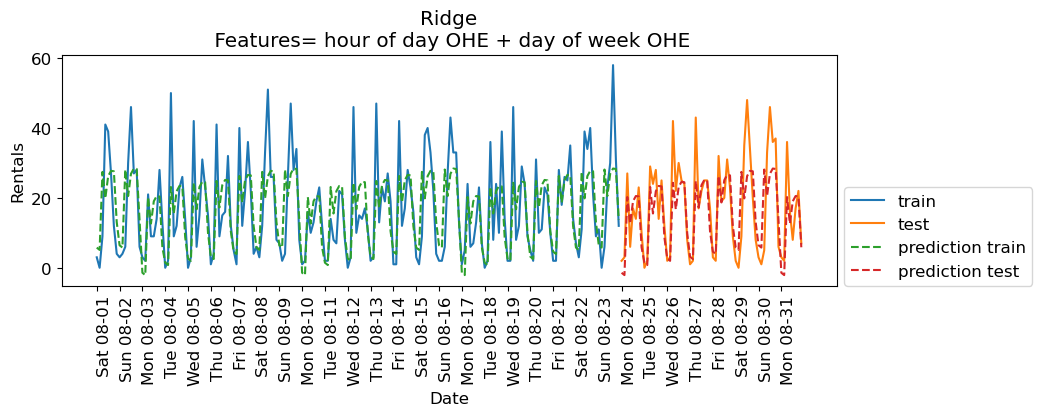
• The scores are a bit better now.

• What if we add interaction features (e.g., something like Day == Mon and hour == 9:00)

• We can do it using sklearn’s PolynomialFeatures transformer.

from sklearn.preprocessing import PolynomialFeatures

poly_transformer = PolynomialFeatures(
    interaction_only=True, include_bias=False
)
X_hour_week_onehot_poly = poly_transformer.fit_transform(X_hour_week_onehot)

hour = ["%02d:00" % i for i in range(0, 24, 3)]
day = ["Mon", "Tue", "Wed", "Thu", "Fri", "Sat", "Sun"]
features = day + hour
features_poly = poly_transformer.get_feature_names_out(features)
features_poly

array(['Mon', 'Tue', 'Wed', 'Thu', 'Fri', 'Sat', 'Sun', '00:00', '03:00',
       '06:00', '09:00', '12:00', '15:00', '18:00', '21:00', 'Mon Tue',
       'Mon Wed', 'Mon Thu', 'Mon Fri', 'Mon Sat', 'Mon Sun', 'Mon 00:00',
       'Mon 03:00', 'Mon 06:00', 'Mon 09:00', 'Mon 12:00', 'Mon 15:00',
       'Mon 18:00', 'Mon 21:00', 'Tue Wed', 'Tue Thu', 'Tue Fri',
       'Tue Sat', 'Tue Sun', 'Tue 00:00', 'Tue 03:00', 'Tue 06:00',
       'Tue 09:00', 'Tue 12:00', 'Tue 15:00', 'Tue 18:00', 'Tue 21:00',
       'Wed Thu', 'Wed Fri', 'Wed Sat', 'Wed Sun', 'Wed 00:00',
       'Wed 03:00', 'Wed 06:00', 'Wed 09:00', 'Wed 12:00', 'Wed 15:00',
       'Wed 18:00', 'Wed 21:00', 'Thu Fri', 'Thu Sat', 'Thu Sun',
       'Thu 00:00', 'Thu 03:00', 'Thu 06:00', 'Thu 09:00', 'Thu 12:00',
       'Thu 15:00', 'Thu 18:00', 'Thu 21:00', 'Fri Sat', 'Fri Sun',
       'Fri 00:00', 'Fri 03:00', 'Fri 06:00', 'Fri 09:00', 'Fri 12:00',
       'Fri 15:00', 'Fri 18:00', 'Fri 21:00', 'Sat Sun', 'Sat 00:00',
       'Sat 03:00', 'Sat 06:00', 'Sat 09:00', 'Sat 12:00', 'Sat 15:00',
       'Sat 18:00', 'Sat 21:00', 'Sun 00:00', 'Sun 03:00', 'Sun 06:00',
       'Sun 09:00', 'Sun 12:00', 'Sun 15:00', 'Sun 18:00', 'Sun 21:00',
       '00:00 03:00', '00:00 06:00', '00:00 09:00', '00:00 12:00',
       '00:00 15:00', '00:00 18:00', '00:00 21:00', '03:00 06:00',
       '03:00 09:00', '03:00 12:00', '03:00 15:00', '03:00 18:00',
       '03:00 21:00', '06:00 09:00', '06:00 12:00', '06:00 15:00',
       '06:00 18:00', '06:00 21:00', '09:00 12:00', '09:00 15:00',
       '09:00 18:00', '09:00 21:00', '12:00 15:00', '12:00 18:00',
       '12:00 21:00', '15:00 18:00', '15:00 21:00', '18:00 21:00'],
      dtype=object)

df_hour_week_ohe_poly = pd.DataFrame(X_hour_week_onehot_poly, columns = features_poly)
df_hour_week_ohe_poly

	Mon	Tue	Wed	Thu	Fri	Sat	Sun	00:00	03:00	06:00	...	09:00 12:00	09:00 15:00	09:00 18:00	09:00 21:00	12:00 15:00	12:00 18:00	12:00 21:00	15:00 18:00	15:00 21:00	18:00 21:00
0	0.0	0.0	0.0	0.0	0.0	1.0	0.0	1.0	0.0	0.0	...	0.0	0.0	0.0	0.0	0.0	0.0	0.0	0.0	0.0	0.0
1	0.0	0.0	0.0	0.0	0.0	1.0	0.0	0.0	1.0	0.0	...	0.0	0.0	0.0	0.0	0.0	0.0	0.0	0.0	0.0	0.0
2	0.0	0.0	0.0	0.0	0.0	1.0	0.0	0.0	0.0	1.0	...	0.0	0.0	0.0	0.0	0.0	0.0	0.0	0.0	0.0	0.0
3	0.0	0.0	0.0	0.0	0.0	1.0	0.0	0.0	0.0	0.0	...	0.0	0.0	0.0	0.0	0.0	0.0	0.0	0.0	0.0	0.0
4	0.0	0.0	0.0	0.0	0.0	1.0	0.0	0.0	0.0	0.0	...	0.0	0.0	0.0	0.0	0.0	0.0	0.0	0.0	0.0	0.0
...	...	...	...	...	...	...	...	...	...	...	...	...	...	...	...	...	...	...	...	...	...
243	1.0	0.0	0.0	0.0	0.0	0.0	0.0	0.0	0.0	0.0	...	0.0	0.0	0.0	0.0	0.0	0.0	0.0	0.0	0.0	0.0
244	1.0	0.0	0.0	0.0	0.0	0.0	0.0	0.0	0.0	0.0	...	0.0	0.0	0.0	0.0	0.0	0.0	0.0	0.0	0.0	0.0
245	1.0	0.0	0.0	0.0	0.0	0.0	0.0	0.0	0.0	0.0	...	0.0	0.0	0.0	0.0	0.0	0.0	0.0	0.0	0.0	0.0
246	1.0	0.0	0.0	0.0	0.0	0.0	0.0	0.0	0.0	0.0	...	0.0	0.0	0.0	0.0	0.0	0.0	0.0	0.0	0.0	0.0
247	1.0	0.0	0.0	0.0	0.0	0.0	0.0	0.0	0.0	0.0	...	0.0	0.0	0.0	0.0	0.0	0.0	0.0	0.0	0.0	0.0

248 rows × 120 columns

X_hour_week_onehot_poly.shape

(248, 120)

lr = Ridge()
eval_on_features(X_hour_week_onehot_poly, y, lr, feat_names = "hour of day OHE + day of week OHE + interaction feats")

Train-set R^2: 0.87
Test-set R^2: 0.85

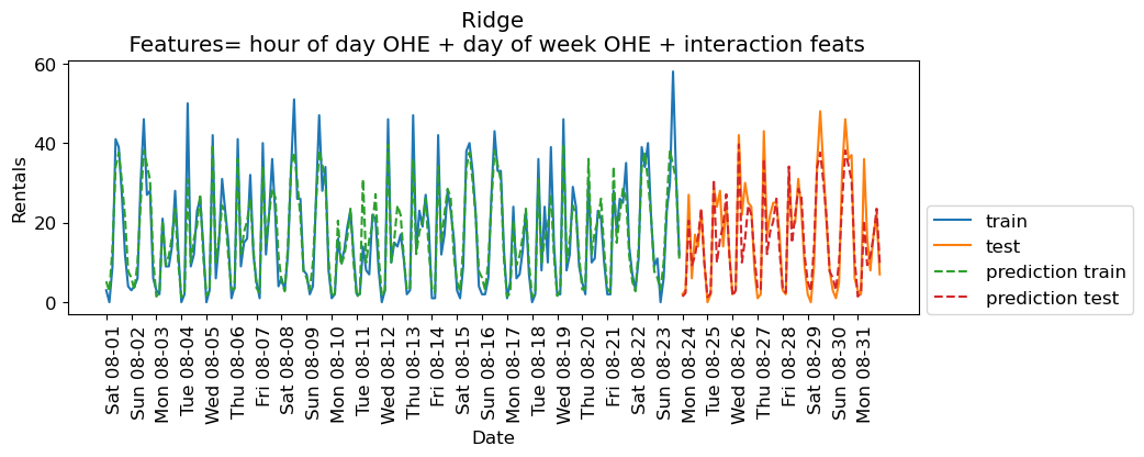
The scores are much better now. Since we are using a linear model, we can examine the coefficients learned by Ridge.

features_nonzero = np.array(features_poly)[lr.coef_ != 0]
coef_nonzero = lr.coef_[lr.coef_ != 0]

pd.DataFrame(coef_nonzero, index=features_nonzero, columns=["Coefficient"]).sort_values(
    "Coefficient", ascending=False
)

	Coefficient
Sat 09:00	15.196739
Wed 06:00	15.005809
Sat 12:00	13.437684
Sun 12:00	13.362009
Thu 06:00	10.907595
...	...
Sat 21:00	-6.085150
00:00	-11.693898
03:00	-12.111220
Sat 06:00	-13.757591
Sun 06:00	-18.033267

71 rows × 1 columns

• The coefficients make sense!

• If it’s Saturday 09:00 or Wednesday 06:00, the model is likely to predict bigger number for rentals.

• If it’s Midnight or 03:00 or Sunday 06:00, the model is likely to predict smaller number for rentals.

Interim summary

• Success in time-series analysis heavily relies on the appropriate choice of models and features.

• Tree-based models cannot extrapolate; caution is needed when using them with linear integer features.

• Linear models struggle with cyclic patterns in numeric features (e.g., numerically encoded time of the day feature) because these patterns are inherently non-linear.

• Applying one-hot encoding on such features transforms cyclic temporal features into a format where their impact on the target variable can be independently and linearly modeled, enabling linear models to effectively capture and use these cyclic patterns.

Lag-based features

• So far we engineered some features and managed to get reasonable results.

• In time series data there is temporal dependence; observations close in time tend to be correlated.

• Currently we’re using current time to predict the number of bike rentals in the next three hours.

• But, what if the number of bike rentals is also related to bike rentals three hours ago or 6 hours ago and so on?

  • Such features are called lagged features.

Note: In time series analysis, you would look at something called an autocorrelation function (ACF), but we won’t go into that here.

Let’s extract lag features. We can “lag” (or “shift”) a time series in Pandas with the .shift() method.

citibike

starttime
2015-08-01 00:00:00     3
2015-08-01 03:00:00     0
2015-08-01 06:00:00     9
2015-08-01 09:00:00    41
2015-08-01 12:00:00    39
                       ..
2015-08-31 09:00:00    16
2015-08-31 12:00:00     8
2015-08-31 15:00:00    17
2015-08-31 18:00:00    22
2015-08-31 21:00:00     7
Freq: 3H, Name: one, Length: 248, dtype: int64

rentals_df = pd.DataFrame(citibike)
rentals_df = rentals_df.rename(columns={"one":"n_rentals"})
rentals_df

	n_rentals
starttime
2015-08-01 00:00:00	3
2015-08-01 03:00:00	0
2015-08-01 06:00:00	9
2015-08-01 09:00:00	41
2015-08-01 12:00:00	39
...	...
2015-08-31 09:00:00	16
2015-08-31 12:00:00	8
2015-08-31 15:00:00	17
2015-08-31 18:00:00	22
2015-08-31 21:00:00	7

248 rows × 1 columns

def create_lag_df(df, lag, cols):
    return df.assign(
        **{f"{col}-{n}": df[col].shift(n) for n in range(1, lag + 1) for col in cols}
    )

rentals_lag5 = create_lag_df(rentals_df, 5, ['n_rentals'] )

rentals_lag5

	n_rentals	n_rentals-1	n_rentals-2	n_rentals-3	n_rentals-4	n_rentals-5
starttime
2015-08-01 00:00:00	3	NaN	NaN	NaN	NaN	NaN
2015-08-01 03:00:00	0	3.0	NaN	NaN	NaN	NaN
2015-08-01 06:00:00	9	0.0	3.0	NaN	NaN	NaN
2015-08-01 09:00:00	41	9.0	0.0	3.0	NaN	NaN
2015-08-01 12:00:00	39	41.0	9.0	0.0	3.0	NaN
...	...	...	...	...	...	...
2015-08-31 09:00:00	16	36.0	2.0	3.0	6.0	37.0
2015-08-31 12:00:00	8	16.0	36.0	2.0	3.0	6.0
2015-08-31 15:00:00	17	8.0	16.0	36.0	2.0	3.0
2015-08-31 18:00:00	22	17.0	8.0	16.0	36.0	2.0
2015-08-31 21:00:00	7	22.0	17.0	8.0	16.0	36.0

248 rows × 6 columns

• Note the NaN pattern.

• We can either drop the first 5 rows or apply imputation. (You have to be careful about )

• Let’s try these features with Ridge model.

X_lag_features = rentals_lag5.drop(columns = ['n_rentals']).to_numpy()
X_lag_features

array([[nan, nan, nan, nan, nan],
       [ 3., nan, nan, nan, nan],
       [ 0.,  3., nan, nan, nan],
       ...,
       [ 8., 16., 36.,  2.,  3.],
       [17.,  8., 16., 36.,  2.],
       [22., 17.,  8., 16., 36.]])

lr = Ridge()
eval_on_features(X_lag_features, y, lr, feat_names="Lag features", impute="yes")

Train-set R^2: 0.25
Test-set R^2: 0.37

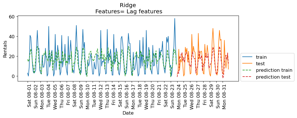
The results are not great. But let’s examine the coefficients.

features_lag = rentals_lag5.drop(columns=['n_rentals']).columns.tolist()
features_nonzero = np.array(features_lag)[lr.coef_ != 0]
coef_nonzero = lr.coef_[lr.coef_ != 0]

pd.DataFrame(coef_nonzero, index=features_nonzero, columns=["Coefficient"]).sort_values(
    "Coefficient", ascending=False
)

	Coefficient
n_rentals-1	0.165617
n_rentals-4	-0.048630
n_rentals-2	-0.214821
n_rentals-3	-0.258225
n_rentals-5	-0.373656

How about RandomForestRegressor model?

imp = SimpleImputer()
X_lag_features_imp = imp.fit_transform(X_lag_features)
rf = RandomForestRegressor()
eval_on_features(X_lag_features_imp, y, rf, feat_names="Lag features")

Train-set R^2: 0.95
Test-set R^2: 0.71

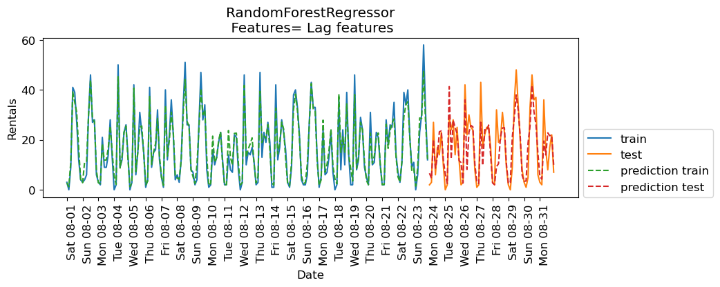
The results are better than Ridge with lag features but they are not as good as the results with our previously engineered features. How about combining lag-based features and the previously extracted features?

X_hour_week_onehot_poly_lag = np.hstack([X_hour_week_onehot_poly, X_lag_features])

rf = RandomForestRegressor()
eval_on_features(X_hour_week_onehot_poly_lag, y, rf, feat_names = "hour of day OHE + day of week OHE + interaction feats + Lag feats")

Train-set R^2: 0.96
Test-set R^2: 0.79

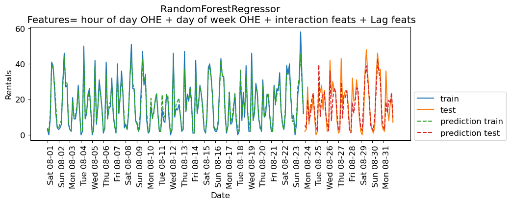
Some improvement but we are getting better results without the lag features in this case.

Cross-validation

What about cross-validation?

• We can’t do regular cross-validation if we don’t want to be predicting the past.

• If you carry out regular cross-validation, as shown below, you’ll be predicting the past given future which is not a realistic scenario for the deployment data.

mglearn.plots.plot_cross_validation()

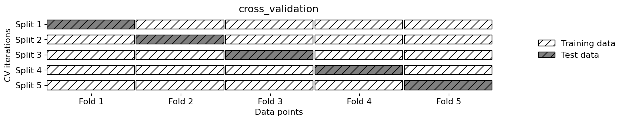
There is TimeSeriesSplit for time series data.

from sklearn.model_selection import TimeSeriesSplit

# Code from sklearn documentation
X_toy = np.array([[1, 2], [3, 4], [1, 2], [3, 4], [1, 2], [3, 4]])
y_toy = np.array([1, 2, 3, 4, 5, 6])
tscv = TimeSeriesSplit(n_splits=3)
for train, test in tscv.split(X_toy):
    print("%s %s" % (train, test))

[0 1 2] [3]
[0 1 2 3] [4]
[0 1 2 3 4] [5]

Let’s try it out with Ridge on the bike rental data.

lr = Ridge()

scores = cross_validate(
    lr, X_hour_week_onehot_poly, y, cv=TimeSeriesSplit(), return_train_score=True
)
pd.DataFrame(scores)

	fit_time	score_time	test_score	train_score
0	0.000866	0.000310	0.642676	0.873182
1	0.000544	0.000221	0.828405	0.874305
2	0.000609	0.000216	0.773851	0.901262
3	0.000622	0.000209	0.696712	0.889429
4	0.001819	0.000785	0.892733	0.863889

Forecasting further into the future

Recall that we are working with the bike rentals data from August 2015.

citibike

starttime
2015-08-01 00:00:00     3
2015-08-01 03:00:00     0
2015-08-01 06:00:00     9
2015-08-01 09:00:00    41
2015-08-01 12:00:00    39
                       ..
2015-08-31 09:00:00    16
2015-08-31 12:00:00     8
2015-08-31 15:00:00    17
2015-08-31 18:00:00    22
2015-08-31 21:00:00     7
Freq: 3H, Name: one, Length: 248, dtype: int64

Here is our data with lag features.

rentals_lag5

	n_rentals	n_rentals-1	n_rentals-2	n_rentals-3	n_rentals-4	n_rentals-5
starttime
2015-08-01 00:00:00	3	NaN	NaN	NaN	NaN	NaN
2015-08-01 03:00:00	0	3.0	NaN	NaN	NaN	NaN
2015-08-01 06:00:00	9	0.0	3.0	NaN	NaN	NaN
2015-08-01 09:00:00	41	9.0	0.0	3.0	NaN	NaN
2015-08-01 12:00:00	39	41.0	9.0	0.0	3.0	NaN
...	...	...	...	...	...	...
2015-08-31 09:00:00	16	36.0	2.0	3.0	6.0	37.0
2015-08-31 12:00:00	8	16.0	36.0	2.0	3.0	6.0
2015-08-31 15:00:00	17	8.0	16.0	36.0	2.0	3.0
2015-08-31 18:00:00	22	17.0	8.0	16.0	36.0	2.0
2015-08-31 21:00:00	7	22.0	17.0	8.0	16.0	36.0

248 rows × 6 columns

Let’s impute the data and create X and y

imp = SimpleImputer()
X_lag_features_imp = imp.fit_transform(X_lag_features)

rentals_lag5_X = pd.DataFrame(X_lag_features_imp, columns=rentals_lag5.drop(columns=['n_rentals']).columns)
rentals_lag5_X.index = rentals_lag5.index
rentals_lag5_X

	n_rentals-1	n_rentals-2	n_rentals-3	n_rentals-4	n_rentals-5
starttime
2015-08-01 00:00:00	17.024291	17.004065	17.004082	17.040984	17.045267
2015-08-01 03:00:00	3.000000	17.004065	17.004082	17.040984	17.045267
2015-08-01 06:00:00	0.000000	3.000000	17.004082	17.040984	17.045267
2015-08-01 09:00:00	9.000000	0.000000	3.000000	17.040984	17.045267
2015-08-01 12:00:00	41.000000	9.000000	0.000000	3.000000	17.045267
...	...	...	...	...	...
2015-08-31 09:00:00	36.000000	2.000000	3.000000	6.000000	37.000000
2015-08-31 12:00:00	16.000000	36.000000	2.000000	3.000000	6.000000
2015-08-31 15:00:00	8.000000	16.000000	36.000000	2.000000	3.000000
2015-08-31 18:00:00	17.000000	8.000000	16.000000	36.000000	2.000000
2015-08-31 21:00:00	22.000000	17.000000	8.000000	16.000000	36.000000

248 rows × 5 columns

rentals_lag5_y = rentals_lag5['n_rentals']

Let’s split the data and train a linear model.

# split the given features into a training and a test set
n_train = 184
X_train, X_test = rentals_lag5_X[:n_train], rentals_lag5_X[n_train:]
# also split the target array
y_train, y_test = rentals_lag5_y[:n_train], rentals_lag5_y[n_train:]

rentals_model = RandomForestRegressor(random_state=42)
rentals_model.fit(X_train, y_train);
print("Train-set R^2: {:.2f}".format(rentals_model.score(X_train, y_train)))
print("Test-set R^2: {:.2f}".format(rentals_model.score(X_test, y_test)))

Train-set R^2: 0.94
Test-set R^2: 0.68

Given this, we can now predict n_rentals on the test data.

X_test

	n_rentals-1	n_rentals-2	n_rentals-3	n_rentals-4	n_rentals-5
starttime
2015-08-24 00:00:00	12.0	31.0	58.0	30.0	23.0
2015-08-24 03:00:00	2.0	12.0	31.0	58.0	30.0
2015-08-24 06:00:00	3.0	2.0	12.0	31.0	58.0
2015-08-24 09:00:00	27.0	3.0	2.0	12.0	31.0
2015-08-24 12:00:00	6.0	27.0	3.0	2.0	12.0
...	...	...	...	...	...
2015-08-31 09:00:00	36.0	2.0	3.0	6.0	37.0
2015-08-31 12:00:00	16.0	36.0	2.0	3.0	6.0
2015-08-31 15:00:00	8.0	16.0	36.0	2.0	3.0
2015-08-31 18:00:00	17.0	8.0	16.0	36.0	2.0
2015-08-31 21:00:00	22.0	17.0	8.0	16.0	36.0

64 rows × 5 columns

preds = rentals_model.predict(X_test)
preds

array([ 6.36,  4.73, 16.84,  8.71, 13.  , 24.34, 23.91, 12.07,  5.44,
        2.11, 42.31, 11.64, 28.09, 26.46, 25.41, 12.28, 11.89,  2.01,
       34.5 ,  8.34, 23.94, 25.2 , 26.63, 11.02,  2.67,  2.71, 26.72,
        9.96, 24.42, 23.05, 26.79, 14.17,  3.22,  1.51,  9.15,  8.83,
       21.12, 24.7 , 25.23, 10.04,  2.21,  2.29, 22.45, 28.03, 36.14,
       32.83, 21.45,  5.8 ,  3.43,  3.18, 21.72, 26.23, 40.37, 34.84,
       27.67, 14.79,  5.44,  4.45, 20.19, 14.49, 23.06, 20.34, 23.02,
       10.11])

X_test_preds = X_test.assign(predicted_n_rentals=preds)
X_test_preds = X_test_preds.assign(n_rentals=y_test)
X_test_preds.tail()

	n_rentals-1	n_rentals-2	n_rentals-3	n_rentals-4	n_rentals-5	predicted_n_rentals	n_rentals
starttime
2015-08-31 09:00:00	36.0	2.0	3.0	6.0	37.0	14.49	16
2015-08-31 12:00:00	16.0	36.0	2.0	3.0	6.0	23.06	8
2015-08-31 15:00:00	8.0	16.0	36.0	2.0	3.0	20.34	17
2015-08-31 18:00:00	17.0	8.0	16.0	36.0	2.0	23.02	22
2015-08-31 21:00:00	22.0	17.0	8.0	16.0	36.0	10.11	7

• Ok, that is fine, but what if we want to predict 15 hours in the future? In other words, what if we want to predict number of rentals for the next three hours at time 2015-09-01 12:00:00?

• Well, we would not have access to our lag features!! We don’t yet know n_rentals for

  • 2015-09-01 00:00:00

  • 2015-09-01 03:00:00

  • 2015-09-01 06:00:00

  • 2015-09-01 09:00:00

There are a few approaches which could be employed:

1. Train a separate model for each number of 3-hour span. E.g. one model that predicts n_rentals for next three hours, another model that predicts n_rentals in six hours, etc. We can build these datasets.

2. Use a multi-output model that jointly predicts n_rentalsIn3hours, n_rentalsIn6hours, etc. However, multi-output models are outside the scope of CPSC 330.

3. Use one model and sequentially predict using a for loop.

If we decide to use approach 3, we would predict these values and then pretend they are true! For example, given that it’s August 31st 2015 at 21:00.

1. Predict n_rentals for September 1st 2015 at 00:00.

2. Then to predict n_rentals for September 1st 2015 at 03:00, we need to know n_rentals for September 1st 2015 at 00:00. Use our prediction for September 1st 2015 at 00:00 as the truth.

3. Then, to predict n_rentals for September 1st 2015 at 06:00, we need to know n_rentals for September 1st 2015 at 00:00 and n_rentals for September 1st 2015 at 03:00. Use our predictions.

4. Etc etc.

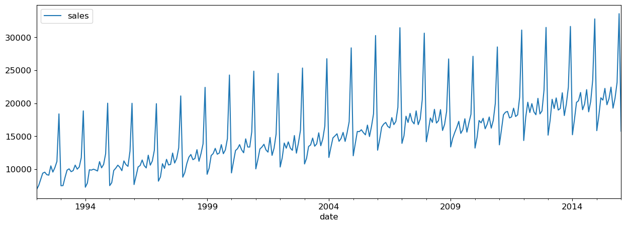
Forecasting further into the future on a retail dataset

Let’s consider another time series dataset, Retail Sales of Clothing and Clothing Accessory Stores dataset which is made available by the Federal Reserve Bank of St. Louis.

The dataset has dates and retail sales values corresponding to the dates.

retail_df = pd.read_csv("data/MRTSSM448USN.csv", parse_dates=["DATE"])
retail_df.columns = ["date", "sales"]

retail_df.head()

	date	sales
0	1992-01-01	6938
1	1992-02-01	7524
2	1992-03-01	8475
3	1992-04-01	9401
4	1992-05-01	9558

Let’s examine the min and max dates in order to split the data.

retail_df["date"].min()

Timestamp('1992-01-01 00:00:00')

retail_df["date"].max()

Timestamp('2022-09-01 00:00:00')

I’m considering everything upto 01 January 2016 as training data and everything after that as test data.

retail_df_train = retail_df.query("date <= 20160101")
retail_df_test = retail_df.query("date >  20160101")

retail_df_train.plot(x="date", y="sales", figsize=(15, 5));

We can create a dataset using purely lag features.

def lag_df(df, lag, cols):
    return df.assign(
        **{f"{col}-{n}": df[col].shift(n) for n in range(1, lag + 1) for col in cols}
    )

Let’s create lag features for the full dataframe.

retail_lag_5 = lag_df(retail_df, 5, ["sales"])

retail_train_5 = retail_lag_5.query("date <= 20160101")
retail_test_5 = retail_lag_5.query("date >  20160101")
retail_train_5

	date	sales	sales-1	sales-2	sales-3	sales-4	sales-5
0	1992-01-01	6938	NaN	NaN	NaN	NaN	NaN
1	1992-02-01	7524	6938.0	NaN	NaN	NaN	NaN
2	1992-03-01	8475	7524.0	6938.0	NaN	NaN	NaN
3	1992-04-01	9401	8475.0	7524.0	6938.0	NaN	NaN
4	1992-05-01	9558	9401.0	8475.0	7524.0	6938.0	NaN
...	...	...	...	...	...	...	...
284	2015-09-01	19266	22452.0	20694.0	19781.0	22260.0	20485.0
285	2015-10-01	20794	19266.0	22452.0	20694.0	19781.0	22260.0
286	2015-11-01	23175	20794.0	19266.0	22452.0	20694.0	19781.0
287	2015-12-01	33590	23175.0	20794.0	19266.0	22452.0	20694.0
288	2016-01-01	15775	33590.0	23175.0	20794.0	19266.0	22452.0

289 rows × 7 columns

• Now, if we drop the “date” column we have a target (“sales”) and 5 features (the previous 5 days of sales).

• We need to impute/drop the missing values and then we can fit a model to this. I will just drop for convenience:

retail_train_5 = retail_train_5[5:].drop(columns=["date"])
retail_train_5

	sales	sales-1	sales-2	sales-3	sales-4	sales-5
5	9182	9558.0	9401.0	8475.0	7524.0	6938.0
6	9103	9182.0	9558.0	9401.0	8475.0	7524.0
7	10513	9103.0	9182.0	9558.0	9401.0	8475.0
8	9573	10513.0	9103.0	9182.0	9558.0	9401.0
9	10254	9573.0	10513.0	9103.0	9182.0	9558.0
...	...	...	...	...	...	...
284	19266	22452.0	20694.0	19781.0	22260.0	20485.0
285	20794	19266.0	22452.0	20694.0	19781.0	22260.0
286	23175	20794.0	19266.0	22452.0	20694.0	19781.0
287	33590	23175.0	20794.0	19266.0	22452.0	20694.0
288	15775	33590.0	23175.0	20794.0	19266.0	22452.0

284 rows × 6 columns

retail_train_5_X = retail_train_5.drop(columns=["sales"])
retail_train_5_y = retail_train_5["sales"]

retail_model = RandomForestRegressor(random_state=42)
retail_model.fit(retail_train_5_X, retail_train_5_y);
print("Train-set R^2: {:.2f}".format(retail_model.score(retail_train_5_X, retail_train_5_y)))

Train-set R^2: 0.96

Given this, we can now predict the sales

retail_test_5

	date	sales	sales-1	sales-2	sales-3	sales-4	sales-5
289	2016-02-01	19032	15775.0	33590.0	23175.0	20794.0	19266.0
290	2016-03-01	21581	19032.0	15775.0	33590.0	23175.0	20794.0
291	2016-04-01	20514	21581.0	19032.0	15775.0	33590.0	23175.0
292	2016-05-01	21774	20514.0	21581.0	19032.0	15775.0	33590.0
293	2016-06-01	20274	21774.0	20514.0	21581.0	19032.0	15775.0
...	...	...	...	...	...	...	...
364	2022-05-01	26831	25904.0	25622.0	20509.0	18113.0	39375.0
365	2022-06-01	25031	26831.0	25904.0	25622.0	20509.0	18113.0
366	2022-07-01	25214	25031.0	26831.0	25904.0	25622.0	20509.0
367	2022-08-01	26376	25214.0	25031.0	26831.0	25904.0	25622.0
368	2022-09-01	23941	26376.0	25214.0	25031.0	26831.0	25904.0

80 rows × 7 columns

preds = retail_model.predict(retail_test_5.drop(columns=["date", "sales"]))
preds

array([17896.8 , 21694.77, 21603.92, 21847.23, 21405.8 , 20564.86,
       22154.04, 26063.73, 21389.05, 22320.42, 30167.05, 16153.78,
       18096.6 , 20310.9 , 21353.73, 22826.97, 21697.73, 21549.23,
       21768.07, 27206.55, 21571.78, 22057.72, 28953.14, 16160.1 ,
       18000.99, 21596.28, 22910.96, 22225.52, 28327.52, 20620.57,
       22114.07, 30279.79, 21605.25, 21668.73, 18313.24, 16153.78,
       18245.22, 20319.6 , 23290.45, 22788.29, 28362.34, 22219.81,
       21530.08, 29881.14, 21617.54, 21670.38, 19380.36, 16157.83,
       18955.53, 22078.43, 13107.93, 11057.81, 10910.98, 15429.94,
       13255.13, 10868.94, 18311.55, 21274.73, 23902.03, 14813.7 ,
       17518.48, 18533.12, 30146.97, 29691.79, 15661.24, 27638.52,
       19365.48, 25176.  , 27021.21, 28854.11, 15915.6 , 16358.48,
       20334.54, 22550.67, 18116.77, 17144.95, 16533.7 , 25037.25,
       19365.48, 17205.11])

retail_test_5_preds = retail_test_5.assign(predicted_sales=preds)
retail_test_5_preds.tail()

	date	sales	sales-1	sales-2	sales-3	sales-4	sales-5	predicted_sales
364	2022-05-01	26831	25904.0	25622.0	20509.0	18113.0	39375.0	17144.95
365	2022-06-01	25031	26831.0	25904.0	25622.0	20509.0	18113.0	16533.70
366	2022-07-01	25214	25031.0	26831.0	25904.0	25622.0	20509.0	25037.25
367	2022-08-01	26376	25214.0	25031.0	26831.0	25904.0	25622.0	19365.48
368	2022-09-01	23941	26376.0	25214.0	25031.0	26831.0	25904.0	17205.11

• Now what if we want to predict 5 months in the future?

• We would not have access to our features!! We don’t yet know the previous months sales, or two months prior!

If we decide to use approach 3 from above, we would predict these values and then pretend they are true! For example, given that it’s November 2022

1. Predict December 2022 sales

2. Then, to predict for January 2023, we need to know December 2022 sales. Use our prediction for December 2022 as the truth.

3. Then, to predict for February 2023, we need to know December 2022 and January 2023 sales. Use our predictions.

4. Etc etc.

Seasonality and trends

• There are some important concepts in time series that rely on having a continuous target (like we do in the retail sales example above).

• Part of that is the idea of seasonality and trends.

• These are mostly taken care of by our feature engineering of the data variable, but there’s something important left to discuss.

retail_df_train.plot(x="date", y="sales", figsize=(15, 5));

• It looks like there’s a trend here - the sales are going up over time.

Let’s say we encoded the date as a feature in days like this:

retail_train_5_date = retail_lag_5.query("date <= 20160101")
first_day_retail = retail_train_5_date["date"].min()

retail_train_5_date = retail_train_5_date.assign(
    Days_since=retail_train_5_date["date"].apply(lambda x: (x - first_day_retail).days)
)
retail_train_5_date.head(10)

	date	sales	sales-1	sales-2	sales-3	sales-4	sales-5	Days_since
0	1992-01-01	6938	NaN	NaN	NaN	NaN	NaN	0
1	1992-02-01	7524	6938.0	NaN	NaN	NaN	NaN	31
2	1992-03-01	8475	7524.0	6938.0	NaN	NaN	NaN	60
3	1992-04-01	9401	8475.0	7524.0	6938.0	NaN	NaN	91
4	1992-05-01	9558	9401.0	8475.0	7524.0	6938.0	NaN	121
5	1992-06-01	9182	9558.0	9401.0	8475.0	7524.0	6938.0	152
6	1992-07-01	9103	9182.0	9558.0	9401.0	8475.0	7524.0	182
7	1992-08-01	10513	9103.0	9182.0	9558.0	9401.0	8475.0	213
8	1992-09-01	9573	10513.0	9103.0	9182.0	9558.0	9401.0	244
9	1992-10-01	10254	9573.0	10513.0	9103.0	9182.0	9558.0	274

• Now, let’s say we use all these features (the lagged version of the target and also Days_since.

• If we use linear regression we’ll learn a coefficient for Days_since.

  • If that coefficient is positive, it predicts unlimited growth forever. That may not be what you want? It depends.

• If we use a random forest, we’ll just be doing splits from the training set, e.g. “if Days_since > 9100 then do this”.

  • There will be no splits for later time points because there is no training data there.

  • Thus tree-based models cannot model trends.

  • This is really important to know!!

• Often, we model the trend separately and use the random forest to model a de-trended time series.

Demo: A more complicated dataset

Rain in Australia dataset. Predicting whether or not it will rain tomorrow based on today’s measurements.

rain_df = pd.read_csv("data/weatherAUS.csv")
rain_df.head()

	Date	Location	MinTemp	MaxTemp	Rainfall	Evaporation	Sunshine	WindGustDir	WindGustSpeed	WindDir9am	...	Humidity9am	Humidity3pm	Pressure9am	Pressure3pm	Cloud9am	Cloud3pm	Temp9am	Temp3pm	RainToday	RainTomorrow
0	2008-12-01	Albury	13.4	22.9	0.6	NaN	NaN	W	44.0	W	...	71.0	22.0	1007.7	1007.1	8.0	NaN	16.9	21.8	No	No
1	2008-12-02	Albury	7.4	25.1	0.0	NaN	NaN	WNW	44.0	NNW	...	44.0	25.0	1010.6	1007.8	NaN	NaN	17.2	24.3	No	No
2	2008-12-03	Albury	12.9	25.7	0.0	NaN	NaN	WSW	46.0	W	...	38.0	30.0	1007.6	1008.7	NaN	2.0	21.0	23.2	No	No
3	2008-12-04	Albury	9.2	28.0	0.0	NaN	NaN	NE	24.0	SE	...	45.0	16.0	1017.6	1012.8	NaN	NaN	18.1	26.5	No	No
4	2008-12-05	Albury	17.5	32.3	1.0	NaN	NaN	W	41.0	ENE	...	82.0	33.0	1010.8	1006.0	7.0	8.0	17.8	29.7	No	No

5 rows × 23 columns

rain_df.shape

(145460, 23)

Questions of interest

• Can we forecast into the future? Can we predict whether it’s going to rain tomorrow?

  • The target variable is RainTomorrow. The target is categorical and not continuous in this case.

• Can the date/time features help us predict the target value?

Exploratory data analysis

rain_df.info()

<class 'pandas.core.frame.DataFrame'>
RangeIndex: 145460 entries, 0 to 145459
Data columns (total 23 columns):
 #   Column         Non-Null Count   Dtype  
---  ------         --------------   -----  
 0   Date           145460 non-null  object 
 1   Location       145460 non-null  object 
 2   MinTemp        143975 non-null  float64
 3   MaxTemp        144199 non-null  float64
 4   Rainfall       142199 non-null  float64
 5   Evaporation    82670 non-null   float64
 6   Sunshine       75625 non-null   float64
 7   WindGustDir    135134 non-null  object 
 8   WindGustSpeed  135197 non-null  float64
 9   WindDir9am     134894 non-null  object 
 10  WindDir3pm     141232 non-null  object 
 11  WindSpeed9am   143693 non-null  float64
 12  WindSpeed3pm   142398 non-null  float64
 13  Humidity9am    142806 non-null  float64
 14  Humidity3pm    140953 non-null  float64
 15  Pressure9am    130395 non-null  float64
 16  Pressure3pm    130432 non-null  float64
 17  Cloud9am       89572 non-null   float64
 18  Cloud3pm       86102 non-null   float64
 19  Temp9am        143693 non-null  float64
 20  Temp3pm        141851 non-null  float64
 21  RainToday      142199 non-null  object 
 22  RainTomorrow   142193 non-null  object 
dtypes: float64(16), object(7)
memory usage: 25.5+ MB

rain_df.describe(include="all")

	Date	Location	MinTemp	MaxTemp	Rainfall	Evaporation	Sunshine	WindGustDir	WindGustSpeed	WindDir9am	...	Humidity9am	Humidity3pm	Pressure9am	Pressure3pm	Cloud9am	Cloud3pm	Temp9am	Temp3pm	RainToday	RainTomorrow
count	145460	145460	143975.000000	144199.000000	142199.000000	82670.000000	75625.000000	135134	135197.000000	134894	...	142806.000000	140953.000000	130395.00000	130432.000000	89572.000000	86102.000000	143693.000000	141851.00000	142199	142193
unique	3436	49	NaN	NaN	NaN	NaN	NaN	16	NaN	16	...	NaN	NaN	NaN	NaN	NaN	NaN	NaN	NaN	2	2
top	2013-11-12	Canberra	NaN	NaN	NaN	NaN	NaN	W	NaN	N	...	NaN	NaN	NaN	NaN	NaN	NaN	NaN	NaN	No	No
freq	49	3436	NaN	NaN	NaN	NaN	NaN	9915	NaN	11758	...	NaN	NaN	NaN	NaN	NaN	NaN	NaN	NaN	110319	110316
mean	NaN	NaN	12.194034	23.221348	2.360918	5.468232	7.611178	NaN	40.035230	NaN	...	68.880831	51.539116	1017.64994	1015.255889	4.447461	4.509930	16.990631	21.68339	NaN	NaN
std	NaN	NaN	6.398495	7.119049	8.478060	4.193704	3.785483	NaN	13.607062	NaN	...	19.029164	20.795902	7.10653	7.037414	2.887159	2.720357	6.488753	6.93665	NaN	NaN
min	NaN	NaN	-8.500000	-4.800000	0.000000	0.000000	0.000000	NaN	6.000000	NaN	...	0.000000	0.000000	980.50000	977.100000	0.000000	0.000000	-7.200000	-5.40000	NaN	NaN
25%	NaN	NaN	7.600000	17.900000	0.000000	2.600000	4.800000	NaN	31.000000	NaN	...	57.000000	37.000000	1012.90000	1010.400000	1.000000	2.000000	12.300000	16.60000	NaN	NaN
50%	NaN	NaN	12.000000	22.600000	0.000000	4.800000	8.400000	NaN	39.000000	NaN	...	70.000000	52.000000	1017.60000	1015.200000	5.000000	5.000000	16.700000	21.10000	NaN	NaN
75%	NaN	NaN	16.900000	28.200000	0.800000	7.400000	10.600000	NaN	48.000000	NaN	...	83.000000	66.000000	1022.40000	1020.000000	7.000000	7.000000	21.600000	26.40000	NaN	NaN
max	NaN	NaN	33.900000	48.100000	371.000000	145.000000	14.500000	NaN	135.000000	NaN	...	100.000000	100.000000	1041.00000	1039.600000	9.000000	9.000000	40.200000	46.70000	NaN	NaN

11 rows × 23 columns

• A number of missing values.

• Some target values are also missing. I’m dropping these rows.

rain_df = rain_df[rain_df["RainTomorrow"].notna()]
rain_df.shape

(142193, 23)

Parsing datetimes

• In general, datetimes are a huge pain!

  • Think of all the formats: MM-DD-YY, DD-MM-YY, YY-MM-DD, MM/DD/YY, DD/MM/YY, DD/MM/YYYY, 20:45, 8:45am, 8:45 PM, 8:45a, 08:00, 8:10:20, …….

  • Time zones.

  • Daylight savings…

• Thankfully, pandas does a pretty good job here.

dates_rain = pd.to_datetime(rain_df["Date"])
dates_rain

0        2008-12-01
1        2008-12-02
2        2008-12-03
3        2008-12-04
4        2008-12-05
            ...    
145454   2017-06-20
145455   2017-06-21
145456   2017-06-22
145457   2017-06-23
145458   2017-06-24
Name: Date, Length: 142193, dtype: datetime64[ns]

They are all the same format, so we can also compare dates:

dates_rain[1] - dates_rain[0] 

Timedelta('1 days 00:00:00')

dates_rain[1] > dates_rain[0]

True

(dates_rain[1] - dates_rain[0]).total_seconds()

86400.0

We can also easily extract information from the date columns.

dates_rain[1]

Timestamp('2008-12-02 00:00:00')

dates_rain[1].month_name()

'December'

dates_rain[1].day_name()

'Tuesday'

dates_rain[1].is_year_end

False

dates_rain[1].is_leap_year

True

Above pandas identified the date column automatically. You can tell pandas to parse the dates when reading in the CSV:

rain_df = pd.read_csv("data/weatherAUS.csv", parse_dates=["Date"])
rain_df.head()

	Date	Location	MinTemp	MaxTemp	Rainfall	Evaporation	Sunshine	WindGustDir	WindGustSpeed	WindDir9am	...	Humidity9am	Humidity3pm	Pressure9am	Pressure3pm	Cloud9am	Cloud3pm	Temp9am	Temp3pm	RainToday	RainTomorrow
0	2008-12-01	Albury	13.4	22.9	0.6	NaN	NaN	W	44.0	W	...	71.0	22.0	1007.7	1007.1	8.0	NaN	16.9	21.8	No	No
1	2008-12-02	Albury	7.4	25.1	0.0	NaN	NaN	WNW	44.0	NNW	...	44.0	25.0	1010.6	1007.8	NaN	NaN	17.2	24.3	No	No
2	2008-12-03	Albury	12.9	25.7	0.0	NaN	NaN	WSW	46.0	W	...	38.0	30.0	1007.6	1008.7	NaN	2.0	21.0	23.2	No	No
3	2008-12-04	Albury	9.2	28.0	0.0	NaN	NaN	NE	24.0	SE	...	45.0	16.0	1017.6	1012.8	NaN	NaN	18.1	26.5	No	No
4	2008-12-05	Albury	17.5	32.3	1.0	NaN	NaN	W	41.0	ENE	...	82.0	33.0	1010.8	1006.0	7.0	8.0	17.8	29.7	No	No

5 rows × 23 columns

rain_df = rain_df[rain_df["RainTomorrow"].notna()]
rain_df.shape

(142193, 23)

rain_df

	Date	Location	MinTemp	MaxTemp	Rainfall	Evaporation	Sunshine	WindGustDir	WindGustSpeed	WindDir9am	...	Humidity9am	Humidity3pm	Pressure9am	Pressure3pm	Cloud9am	Cloud3pm	Temp9am	Temp3pm	RainToday	RainTomorrow
0	2008-12-01	Albury	13.4	22.9	0.6	NaN	NaN	W	44.0	W	...	71.0	22.0	1007.7	1007.1	8.0	NaN	16.9	21.8	No	No
1	2008-12-02	Albury	7.4	25.1	0.0	NaN	NaN	WNW	44.0	NNW	...	44.0	25.0	1010.6	1007.8	NaN	NaN	17.2	24.3	No	No
2	2008-12-03	Albury	12.9	25.7	0.0	NaN	NaN	WSW	46.0	W	...	38.0	30.0	1007.6	1008.7	NaN	2.0	21.0	23.2	No	No
3	2008-12-04	Albury	9.2	28.0	0.0	NaN	NaN	NE	24.0	SE	...	45.0	16.0	1017.6	1012.8	NaN	NaN	18.1	26.5	No	No
4	2008-12-05	Albury	17.5	32.3	1.0	NaN	NaN	W	41.0	ENE	...	82.0	33.0	1010.8	1006.0	7.0	8.0	17.8	29.7	No	No
...	...	...	...	...	...	...	...	...	...	...	...	...	...	...	...	...	...	...	...	...	...
145454	2017-06-20	Uluru	3.5	21.8	0.0	NaN	NaN	E	31.0	ESE	...	59.0	27.0	1024.7	1021.2	NaN	NaN	9.4	20.9	No	No
145455	2017-06-21	Uluru	2.8	23.4	0.0	NaN	NaN	E	31.0	SE	...	51.0	24.0	1024.6	1020.3	NaN	NaN	10.1	22.4	No	No
145456	2017-06-22	Uluru	3.6	25.3	0.0	NaN	NaN	NNW	22.0	SE	...	56.0	21.0	1023.5	1019.1	NaN	NaN	10.9	24.5	No	No
145457	2017-06-23	Uluru	5.4	26.9	0.0	NaN	NaN	N	37.0	SE	...	53.0	24.0	1021.0	1016.8	NaN	NaN	12.5	26.1	No	No
145458	2017-06-24	Uluru	7.8	27.0	0.0	NaN	NaN	SE	28.0	SSE	...	51.0	24.0	1019.4	1016.5	3.0	2.0	15.1	26.0	No	No

142193 rows × 23 columns

rain_df.sort_values(by="Date").head()

	Date	Location	MinTemp	MaxTemp	Rainfall	Evaporation	Sunshine	WindGustDir	WindGustSpeed	WindDir9am	...	Humidity9am	Humidity3pm	Pressure9am	Pressure3pm	Cloud9am	Cloud3pm	Temp9am	Temp3pm	RainToday	RainTomorrow
45587	2007-11-01	Canberra	8.0	24.3	0.0	3.4	6.3	NW	30.0	SW	...	68.0	29.0	1019.7	1015.0	7.0	7.0	14.4	23.6	No	Yes
45588	2007-11-02	Canberra	14.0	26.9	3.6	4.4	9.7	ENE	39.0	E	...	80.0	36.0	1012.4	1008.4	5.0	3.0	17.5	25.7	Yes	Yes
45589	2007-11-03	Canberra	13.7	23.4	3.6	5.8	3.3	NW	85.0	N	...	82.0	69.0	1009.5	1007.2	8.0	7.0	15.4	20.2	Yes	Yes
45590	2007-11-04	Canberra	13.3	15.5	39.8	7.2	9.1	NW	54.0	WNW	...	62.0	56.0	1005.5	1007.0	2.0	7.0	13.5	14.1	Yes	Yes
45591	2007-11-05	Canberra	7.6	16.1	2.8	5.6	10.6	SSE	50.0	SSE	...	68.0	49.0	1018.3	1018.5	7.0	7.0	11.1	15.4	Yes	No

5 rows × 23 columns

rain_df.sort_values(by="Date", ascending=False).head()

	Date	Location	MinTemp	MaxTemp	Rainfall	Evaporation	Sunshine	WindGustDir	WindGustSpeed	WindDir9am	...	Humidity9am	Humidity3pm	Pressure9am	Pressure3pm	Cloud9am	Cloud3pm	Temp9am	Temp3pm	RainToday	RainTomorrow
6048	2017-06-25	BadgerysCreek	0.8	18.6	0.2	NaN	NaN	WSW	31.0	NaN	...	99.0	40.0	1018.8	1015.5	NaN	NaN	6.9	17.8	No	No
93279	2017-06-25	GoldCoast	12.9	22.4	0.0	NaN	NaN	NNE	26.0	W	...	66.0	64.0	1020.2	1017.3	NaN	NaN	18.2	21.7	No	No
55101	2017-06-25	MountGinini	-5.3	1.9	0.0	NaN	NaN	WSW	70.0	SW	...	96.0	94.0	NaN	NaN	NaN	NaN	-3.2	0.4	No	No
96319	2017-06-25	Townsville	16.5	25.8	0.0	NaN	NaN	ESE	31.0	SE	...	61.0	53.0	1018.1	1015.7	8.0	8.0	22.4	24.6	No	No
52061	2017-06-25	Tuggeranong	-5.8	14.4	0.0	NaN	NaN	W	43.0	SSE	...	86.0	49.0	1018.5	1016.0	NaN	NaN	-0.5	11.3	No	No

5 rows × 23 columns

❓❓ Questions for you

How many time series are present in this dataset?

We definitely see measurements on the same day at different locations.

rain_df.sort_values(by=["Location", "Date"]).head()

	Date	Location	MinTemp	MaxTemp	Rainfall	Evaporation	Sunshine	WindGustDir	WindGustSpeed	WindDir9am	...	Humidity9am	Humidity3pm	Pressure9am	Pressure3pm	Cloud9am	Cloud3pm	Temp9am	Temp3pm	RainToday	RainTomorrow
96320	2008-07-01	Adelaide	8.8	15.7	5.0	1.6	2.6	NW	48.0	SW	...	92.0	67.0	1017.4	1017.7	NaN	NaN	13.5	14.9	Yes	No
96321	2008-07-02	Adelaide	12.7	15.8	0.8	1.4	7.8	SW	35.0	SSW	...	75.0	52.0	1022.4	1022.6	NaN	NaN	13.7	15.5	No	No
96322	2008-07-03	Adelaide	6.2	15.1	0.0	1.8	2.1	W	20.0	NNE	...	81.0	56.0	1027.8	1026.5	NaN	NaN	9.3	13.9	No	No
96323	2008-07-04	Adelaide	5.3	15.9	0.0	1.4	8.0	NNE	30.0	NNE	...	71.0	46.0	1028.7	1025.6	NaN	NaN	10.2	15.3	No	No
96325	2008-07-06	Adelaide	11.3	15.7	NaN	NaN	1.5	NNW	52.0	NNE	...	62.0	62.0	1019.5	1016.2	NaN	NaN	13.0	14.4	NaN	Yes

5 rows × 23 columns

Great! Now we gave a sequence of dates with single row per date. We have a separate timeseries for each region.

Do we have equally spaced measurements?

count = 0 
for name, group in rain_df.groupby(['Location']):
    print("%-30s %s" % (name, group["Date"].sort_values().diff().value_counts()))
    print('\n\n\n')
    count+=1
    if count == 2: 
        break

('Adelaide',)                  Date
1 days     3016
2 days       42
3 days       24
4 days        4
31 days       1
32 days       1
29 days       1
Name: count, dtype: int64




('Albany',)                    Date
1 days     2993
2 days       15
3 days        4
31 days       1
33 days       1
29 days       1
Name: count, dtype: int64

The typical spacing seems to be 1 day for each location but there are several exceptions. We seem to have several missing measurements.

Train/test splits

Remember that we should not be calling the usual train_test_split with shuffling because if we want to forecast, we aren’t allowed to know what happened in the future!

rain_df["Date"].min()

Timestamp('2007-11-01 00:00:00')

rain_df["Date"].max()

Timestamp('2017-06-25 00:00:00')

• It looks like we have 10 years of data.

• Let’s use the last 2 years for test.

train_df = rain_df.query("Date <= 20150630")
test_df = rain_df.query("Date >  20150630")

len(train_df)

107502

len(test_df)

34691

len(test_df) / (len(train_df) + len(test_df))

0.24397122221206388

As we can see, we’re still using about 25% of our data as test data.

train_df_sort = train_df.query("Location == 'Sydney'").sort_values(by="Date")
test_df_sort = test_df.query("Location == 'Sydney'").sort_values(by="Date")

plt.figure(figsize=(5,4))
plt.plot(train_df_sort["Date"], train_df_sort["Rainfall"], "b", label="train")
plt.plot(test_df_sort["Date"], test_df_sort["Rainfall"], "r", label="test")
plt.xticks(rotation="vertical")
plt.legend()
plt.ylabel("Rainfall (mm)")
plt.title("Train/test rainfall in Sydney");

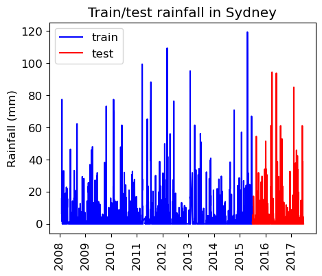
We’re learning relationships from the blue part; predicting only using features in the red part from the day before.

Preprocessing

We have different types of features. So let’s define a preprocessor with a column transformer.

train_df.head()

	Date	Location	MinTemp	MaxTemp	Rainfall	Evaporation	Sunshine	WindGustDir	WindGustSpeed	WindDir9am	...	Humidity9am	Humidity3pm	Pressure9am	Pressure3pm	Cloud9am	Cloud3pm	Temp9am	Temp3pm	RainToday	RainTomorrow
0	2008-12-01	Albury	13.4	22.9	0.6	NaN	NaN	W	44.0	W	...	71.0	22.0	1007.7	1007.1	8.0	NaN	16.9	21.8	No	No
1	2008-12-02	Albury	7.4	25.1	0.0	NaN	NaN	WNW	44.0	NNW	...	44.0	25.0	1010.6	1007.8	NaN	NaN	17.2	24.3	No	No
2	2008-12-03	Albury	12.9	25.7	0.0	NaN	NaN	WSW	46.0	W	...	38.0	30.0	1007.6	1008.7	NaN	2.0	21.0	23.2	No	No
3	2008-12-04	Albury	9.2	28.0	0.0	NaN	NaN	NE	24.0	SE	...	45.0	16.0	1017.6	1012.8	NaN	NaN	18.1	26.5	No	No
4	2008-12-05	Albury	17.5	32.3	1.0	NaN	NaN	W	41.0	ENE	...	82.0	33.0	1010.8	1006.0	7.0	8.0	17.8	29.7	No	No

5 rows × 23 columns

train_df.columns

Index(['Date', 'Location', 'MinTemp', 'MaxTemp', 'Rainfall', 'Evaporation',
       'Sunshine', 'WindGustDir', 'WindGustSpeed', 'WindDir9am', 'WindDir3pm',
       'WindSpeed9am', 'WindSpeed3pm', 'Humidity9am', 'Humidity3pm',
       'Pressure9am', 'Pressure3pm', 'Cloud9am', 'Cloud3pm', 'Temp9am',
       'Temp3pm', 'RainToday', 'RainTomorrow'],
      dtype='object')

train_df.info()

<class 'pandas.core.frame.DataFrame'>
Index: 107502 entries, 0 to 144733
Data columns (total 23 columns):
 #   Column         Non-Null Count   Dtype         
---  ------         --------------   -----         
 0   Date           107502 non-null  datetime64[ns]
 1   Location       107502 non-null  object        
 2   MinTemp        107050 non-null  float64       
 3   MaxTemp        107292 non-null  float64       
 4   Rainfall       106424 non-null  float64       
 5   Evaporation    66221 non-null   float64       
 6   Sunshine       62320 non-null   float64       
 7   WindGustDir    100103 non-null  object        
 8   WindGustSpeed  100146 non-null  float64       
 9   WindDir9am     99515 non-null   object        
 10  WindDir3pm     105314 non-null  object        
 11  WindSpeed9am   106322 non-null  float64       
 12  WindSpeed3pm   106319 non-null  float64       
 13  Humidity9am    106112 non-null  float64       
 14  Humidity3pm    106180 non-null  float64       
 15  Pressure9am    97217 non-null   float64       
 16  Pressure3pm    97253 non-null   float64       
 17  Cloud9am       68523 non-null   float64       
 18  Cloud3pm       67501 non-null   float64       
 19  Temp9am        106705 non-null  float64       
 20  Temp3pm        106816 non-null  float64       
 21  RainToday      106424 non-null  object        
 22  RainTomorrow   107502 non-null  object        
dtypes: datetime64[ns](1), float64(16), object(6)
memory usage: 19.7+ MB

• We have missing data.

• We have categorical features and numeric features.

• Let’s define feature types.

• Let’s start with dropping the date column and treating it as a usual supervised machine learning problem.

numeric_features = [
    "MinTemp",
    "MaxTemp",
    "Rainfall",
    "Evaporation",
    "Sunshine",
    "WindGustSpeed",
    "WindSpeed9am",
    "WindSpeed3pm",
    "Humidity9am",
    "Humidity3pm",
    "Pressure9am",
    "Pressure3pm",
    "Cloud9am",
    "Cloud3pm",
    "Temp9am",
    "Temp3pm",
]
categorical_features = [
    "Location",
    "WindGustDir",
    "WindDir9am",
    "WindDir3pm",
    "RainToday",
]
drop_features = ["Date"]
target = ["RainTomorrow"]

We’ll be doing feature engineering and preprocessing features several times. So I’ve written a function for preprocessing.

def preprocess_features(
    train_df,
    test_df,
    numeric_features,
    categorical_features,
    drop_features,
    target
):

    all_features = set(numeric_features + categorical_features + drop_features + target)
    if set(train_df.columns) != all_features:
        print("Missing columns", set(train_df.columns) - all_features)
        print("Extra columns", all_features - set(train_df.columns))
        raise Exception("Columns do not match")

    numeric_transformer = make_pipeline(
        SimpleImputer(strategy="median"), StandardScaler()
    )
    categorical_transformer = make_pipeline(
        SimpleImputer(strategy="constant", fill_value="missing"),
        OneHotEncoder(handle_unknown="ignore", sparse_output=False),
    )

    preprocessor = make_column_transformer(
        (numeric_transformer, numeric_features),
        (categorical_transformer, categorical_features),
        ("drop", drop_features),
    )
    preprocessor.fit(train_df)
    ohe_feature_names = (
        preprocessor.named_transformers_["pipeline-2"]
        .named_steps["onehotencoder"]
        .get_feature_names_out(categorical_features)
        .tolist()
    )
    new_columns = numeric_features + ohe_feature_names

    X_train_enc = pd.DataFrame(
        preprocessor.transform(train_df), index=train_df.index, columns=new_columns
    )
    X_test_enc = pd.DataFrame(
        preprocessor.transform(test_df), index=test_df.index, columns=new_columns
    )

    y_train = train_df["RainTomorrow"]
    y_test = test_df["RainTomorrow"]

    return X_train_enc, y_train, X_test_enc, y_test, preprocessor

X_train_enc, y_train, X_test_enc, y_test, preprocessor = preprocess_features(
    train_df,
    test_df,
    numeric_features,
    categorical_features,
    drop_features, target
)

X_train_enc.head()

	MinTemp	MaxTemp	Rainfall	Evaporation	Sunshine	WindGustSpeed	WindSpeed9am	WindSpeed3pm	Humidity9am	Humidity3pm	...	WindDir3pm_SSE	WindDir3pm_SSW	WindDir3pm_SW	WindDir3pm_W	WindDir3pm_WNW	WindDir3pm_WSW	WindDir3pm_missing	RainToday_No	RainToday_Yes	RainToday_missing
0	0.204302	-0.027112	-0.205323	-0.140641	0.160729	0.298612	0.666166	0.599894	0.115428	-1.433514	...	0.0	0.0	0.0	0.0	1.0	0.0	0.0	1.0	0.0	0.0
1	-0.741037	0.287031	-0.275008	-0.140641	0.160729	0.298612	-1.125617	0.373275	-1.314929	-1.288002	...	0.0	0.0	0.0	0.0	0.0	1.0	0.0	1.0	0.0	0.0
2	0.125523	0.372706	-0.275008	-0.140641	0.160729	0.450132	0.554180	0.826513	-1.632786	-1.045481	...	0.0	0.0	0.0	0.0	0.0	1.0	0.0	1.0	0.0	0.0
3	-0.457435	0.701128	-0.275008	-0.140641	0.160729	-1.216596	-0.341712	-1.099749	-1.261953	-1.724539	...	0.0	0.0	0.0	0.0	0.0	0.0	0.0	1.0	0.0	0.0
4	0.850283	1.315134	-0.158867	-0.140641	0.160729	0.071330	-0.789657	0.146656	0.698167	-0.899969	...	0.0	0.0	0.0	0.0	0.0	0.0	0.0	1.0	0.0	0.0

5 rows × 119 columns

DummyClassifier

dc = DummyClassifier()
dc.fit(X_train_enc, y_train);

dc.score(X_train_enc, y_train)

0.7750553478074826

y_train.value_counts()

RainTomorrow
No     83320
Yes    24182
Name: count, dtype: int64

dc.score(X_test_enc, y_test)

0.7781845435415525

LogisticRegression

The function below trains a logistic regression model on the train set, reports train and test scores, and returns learned coefficients as a dataframe.

def score_lr_print_coeff(preprocessor, train_df, y_train, test_df, y_test, X_train_enc):
    lr_pipe = make_pipeline(preprocessor, LogisticRegression(max_iter=1000))
    lr_pipe.fit(train_df, y_train)
    print("Train score: {:.2f}".format(lr_pipe.score(train_df, y_train)))
    print("Test score: {:.2f}".format(lr_pipe.score(test_df, y_test)))
    lr_coef = pd.DataFrame(
        data=lr_pipe.named_steps["logisticregression"].coef_.flatten(),
        index=X_train_enc.columns,
        columns=["Coef"],
    )
    return lr_coef.sort_values(by="Coef", ascending=False)

score_lr_print_coeff(preprocessor, train_df, y_train, test_df, y_test, X_train_enc)

Train score: 0.85
Test score: 0.84

	Coef
Humidity3pm	1.243212
RainToday_missing	0.927576
Pressure9am	0.865455
Location_Witchcliffe	0.729178
WindGustSpeed	0.720396
...	...
Location_Townsville	-0.718523
Location_Katherine	-0.726349
Location_Wollongong	-0.748329
Location_MountGinini	-0.964628
Pressure3pm	-1.221788

119 rows × 1 columns

Cross-validation

• We can carry out cross-validation using TimeSeriesSplit.

• However, things are actually more complicated here because this dataset has multiple time series, one per location.

train_df

	Date	Location	MinTemp	MaxTemp	Rainfall	Evaporation	Sunshine	WindGustDir	WindGustSpeed	WindDir9am	...	Humidity9am	Humidity3pm	Pressure9am	Pressure3pm	Cloud9am	Cloud3pm	Temp9am	Temp3pm	RainToday	RainTomorrow
0	2008-12-01	Albury	13.4	22.9	0.6	NaN	NaN	W	44.0	W	...	71.0	22.0	1007.7	1007.1	8.0	NaN	16.9	21.8	No	No
1	2008-12-02	Albury	7.4	25.1	0.0	NaN	NaN	WNW	44.0	NNW	...	44.0	25.0	1010.6	1007.8	NaN	NaN	17.2	24.3	No	No
2	2008-12-03	Albury	12.9	25.7	0.0	NaN	NaN	WSW	46.0	W	...	38.0	30.0	1007.6	1008.7	NaN	2.0	21.0	23.2	No	No
3	2008-12-04	Albury	9.2	28.0	0.0	NaN	NaN	NE	24.0	SE	...	45.0	16.0	1017.6	1012.8	NaN	NaN	18.1	26.5	No	No
4	2008-12-05	Albury	17.5	32.3	1.0	NaN	NaN	W	41.0	ENE	...	82.0	33.0	1010.8	1006.0	7.0	8.0	17.8	29.7	No	No
...	...	...	...	...	...	...	...	...	...	...	...	...	...	...	...	...	...	...	...	...	...
144729	2015-06-26	Uluru	3.8	18.3	0.0	NaN	NaN	E	39.0	ESE	...	73.0	37.0	1031.5	1027.6	NaN	NaN	8.8	17.2	No	No
144730	2015-06-27	Uluru	2.5	17.1	0.0	NaN	NaN	E	41.0	ESE	...	69.0	40.0	1029.9	1026.0	NaN	NaN	7.0	15.7	No	No
144731	2015-06-28	Uluru	4.5	19.6	0.0	NaN	NaN	ENE	35.0	ESE	...	69.0	39.0	1028.7	1025.0	NaN	3.0	8.9	18.0	No	No
144732	2015-06-29	Uluru	7.6	22.0	0.0	NaN	NaN	ESE	33.0	SE	...	67.0	37.0	1027.2	1023.8	6.0	7.0	11.7	21.5	No	No
144733	2015-06-30	Uluru	6.8	21.1	0.0	NaN	NaN	ESE	35.0	ESE	...	81.0	35.0	1028.6	1025.2	3.0	NaN	10.6	20.2	No	No

107502 rows × 23 columns

train_df.sort_values(by=["Date", "Location"]).head()

	Date	Location	MinTemp	MaxTemp	Rainfall	Evaporation	Sunshine	WindGustDir	WindGustSpeed	WindDir9am	...	Humidity9am	Humidity3pm	Pressure9am	Pressure3pm	Cloud9am	Cloud3pm	Temp9am	Temp3pm	RainToday	RainTomorrow
45587	2007-11-01	Canberra	8.0	24.3	0.0	3.4	6.3	NW	30.0	SW	...	68.0	29.0	1019.7	1015.0	7.0	7.0	14.4	23.6	No	Yes
45588	2007-11-02	Canberra	14.0	26.9	3.6	4.4	9.7	ENE	39.0	E	...	80.0	36.0	1012.4	1008.4	5.0	3.0	17.5	25.7	Yes	Yes
45589	2007-11-03	Canberra	13.7	23.4	3.6	5.8	3.3	NW	85.0	N	...	82.0	69.0	1009.5	1007.2	8.0	7.0	15.4	20.2	Yes	Yes
45590	2007-11-04	Canberra	13.3	15.5	39.8	7.2	9.1	NW	54.0	WNW	...	62.0	56.0	1005.5	1007.0	2.0	7.0	13.5	14.1	Yes	Yes
45591	2007-11-05	Canberra	7.6	16.1	2.8	5.6	10.6	SSE	50.0	SSE	...	68.0	49.0	1018.3	1018.5	7.0	7.0	11.1	15.4	Yes	No

5 rows × 23 columns

• The dataframe is sorted by location and then time.

• Our approach today will be to ignore the fact that we have multiple time series and just OHE the location

• We’ll have multiple measurements for a given timestamp, and that’s OK.

• But, TimeSeriesSplit expects the dataframe to be sorted by date so…

train_df_ordered = train_df.sort_values(by=["Date"])
y_train_ordered = train_df_ordered["RainTomorrow"]

train_df_ordered

	Date	Location	MinTemp	MaxTemp	Rainfall	Evaporation	Sunshine	WindGustDir	WindGustSpeed	WindDir9am	...	Humidity9am	Humidity3pm	Pressure9am	Pressure3pm	Cloud9am	Cloud3pm	Temp9am	Temp3pm	RainToday	RainTomorrow
45587	2007-11-01	Canberra	8.0	24.3	0.0	3.4	6.3	NW	30.0	SW	...	68.0	29.0	1019.7	1015.0	7.0	7.0	14.4	23.6	No	Yes
45588	2007-11-02	Canberra	14.0	26.9	3.6	4.4	9.7	ENE	39.0	E	...	80.0	36.0	1012.4	1008.4	5.0	3.0	17.5	25.7	Yes	Yes
45589	2007-11-03	Canberra	13.7	23.4	3.6	5.8	3.3	NW	85.0	N	...	82.0	69.0	1009.5	1007.2	8.0	7.0	15.4	20.2	Yes	Yes
45590	2007-11-04	Canberra	13.3	15.5	39.8	7.2	9.1	NW	54.0	WNW	...	62.0	56.0	1005.5	1007.0	2.0	7.0	13.5	14.1	Yes	Yes
45591	2007-11-05	Canberra	7.6	16.1	2.8	5.6	10.6	SSE	50.0	SSE	...	68.0	49.0	1018.3	1018.5	7.0	7.0	11.1	15.4	Yes	No
...	...	...	...	...	...	...	...	...	...	...	...	...	...	...	...	...	...	...	...	...	...
57415	2015-06-30	Ballarat	-0.3	10.5	0.0	NaN	NaN	S	26.0	NaN	...	99.0	63.0	1029.5	1027.7	NaN	8.0	4.7	9.3	No	No
119911	2015-06-30	PerthAirport	10.1	23.5	0.0	3.2	5.8	NNE	31.0	NE	...	48.0	33.0	1023.6	1021.7	7.0	6.0	13.3	22.2	No	No
60455	2015-06-30	Bendigo	0.3	11.4	0.0	NaN	NaN	W	19.0	NaN	...	89.0	56.0	1029.3	1027.4	8.0	7.0	6.4	10.5	No	No
66473	2015-06-30	MelbourneAirport	3.2	13.2	0.0	0.8	3.9	N	20.0	N	...	91.0	50.0	1029.6	1027.3	2.0	7.0	5.3	11.9	No	No
144733	2015-06-30	Uluru	6.8	21.1	0.0	NaN	NaN	ESE	35.0	ESE	...	81.0	35.0	1028.6	1025.2	3.0	NaN	10.6	20.2	No	No

107502 rows × 23 columns

lr_pipe = make_pipeline(preprocessor, LogisticRegression(max_iter=1000))
cross_val_score(lr_pipe, train_df_ordered, y_train_ordered, cv=TimeSeriesSplit()).mean()

0.8478874811631412

Feature engineering: Encoding date/time as feature(s)

• Can we use the Date to help us predict the target?

• Probably! E.g. different amounts of rain in different seasons.

• This is feature engineering!

Encoding time as a number

• Idea 1: create a column of “days since Nov 1, 2007”.

train_df = rain_df.query("Date <= 20150630")
test_df = rain_df.query("Date >  20150630")

first_day = train_df["Date"].min()

train_df = train_df.assign(
    Days_since=train_df["Date"].apply(lambda x: (x - first_day).days)
)
test_df = test_df.assign(
    Days_since=test_df["Date"].apply(lambda x: (x - first_day).days)
)

train_df.sort_values(by="Date").head()

	Date	Location	MinTemp	MaxTemp	Rainfall	Evaporation	Sunshine	WindGustDir	WindGustSpeed	WindDir9am	...	Humidity3pm	Pressure9am	Pressure3pm	Cloud9am	Cloud3pm	Temp9am	Temp3pm	RainToday	RainTomorrow	Days_since
45587	2007-11-01	Canberra	8.0	24.3	0.0	3.4	6.3	NW	30.0	SW	...	29.0	1019.7	1015.0	7.0	7.0	14.4	23.6	No	Yes	0
45588	2007-11-02	Canberra	14.0	26.9	3.6	4.4	9.7	ENE	39.0	E	...	36.0	1012.4	1008.4	5.0	3.0	17.5	25.7	Yes	Yes	1
45589	2007-11-03	Canberra	13.7	23.4	3.6	5.8	3.3	NW	85.0	N	...	69.0	1009.5	1007.2	8.0	7.0	15.4	20.2	Yes	Yes	2
45590	2007-11-04	Canberra	13.3	15.5	39.8	7.2	9.1	NW	54.0	WNW	...	56.0	1005.5	1007.0	2.0	7.0	13.5	14.1	Yes	Yes	3
45591	2007-11-05	Canberra	7.6	16.1	2.8	5.6	10.6	SSE	50.0	SSE	...	49.0	1018.3	1018.5	7.0	7.0	11.1	15.4	Yes	No	4

5 rows × 24 columns

X_train_enc, y_train, X_test_enc, y_test, preprocessor = preprocess_features(
    train_df,
    test_df,
    numeric_features + ["Days_since"],
    categorical_features,
    drop_features,
    target
)

score_lr_print_coeff(preprocessor, train_df, y_train, test_df, y_test, X_train_enc)

Train score: 0.85
Test score: 0.84

	Coef
Humidity3pm	1.243125
RainToday_missing	0.939310
Pressure9am	0.864369
Location_Witchcliffe	0.731127
WindGustSpeed	0.720150
...	...
Location_Townsville	-0.715836
Location_Katherine	-0.736917
Location_Wollongong	-0.745582
Location_MountGinini	-0.963181
Pressure3pm	-1.221646

120 rows × 1 columns

• Not much improvement in the scores

• Can you think of other ways to generate features from the Date column?

• What about the month - that seems relevant. How should we encode the month?

Encode it as a categorical variable?

One-hot encoding of the month

train_df = rain_df.query("Date <= 20150630")
test_df = rain_df.query("Date >  20150630")

train_df = train_df.assign(
    Month=train_df["Date"].apply(lambda x: x.month_name())
)  # x.month_name() to get the actual string
test_df = test_df.assign(Month=test_df["Date"].apply(lambda x: x.month_name()))

train_df[["Date", "Month"]].sort_values(by="Month")

	Date	Month
62657	2013-04-14	April
115089	2010-04-15	April
115090	2010-04-16	April
115091	2010-04-17	April
115092	2010-04-18	April
...	...	...
128828	2014-09-20	September
128829	2014-09-21	September
128830	2014-09-22	September
128820	2014-09-12	September
72036	2013-09-29	September

107502 rows × 2 columns

X_train_enc, y_train, X_test_enc, y_test, preprocessor = preprocess_features(
    train_df, test_df, 
    numeric_features, 
    categorical_features + ["Month"], 
    drop_features,
    target
)

score_lr_print_coeff(preprocessor, train_df, y_train, test_df, y_test, X_train_enc)

Train score: 0.85
Test score: 0.84

	Coef
Humidity3pm	1.266912
RainToday_missing	0.945668
Pressure9am	0.798893
Location_Witchcliffe	0.748824
WindGustSpeed	0.705665
...	...
Location_Darwin	-0.735386
Location_Wollongong	-0.748457
Location_Townsville	-0.902783
Location_Katherine	-0.926680
Pressure3pm	-1.181793

131 rows × 1 columns

No change in the results.

One-hot encoding seasons

How about just summer/winter as a feature?

def get_season(month):
    # remember this is Australia
    WINTER_MONTHS = ["June", "July", "August"] 
    AUTUMN_MONTHS = ["March", "April", "May"]
    SUMMER_MONTHS = ["December", "January", "February"]
    SPRING_MONTHS = ["September", "October", "November"]
    if month in WINTER_MONTHS:
        return "Winter"
    elif month in AUTUMN_MONTHS:
        return "Autumn"
    elif month in SUMMER_MONTHS:
        return "Summer"
    else:
        return "Fall"

train_df = train_df.assign(Season=train_df["Month"].apply(get_season))
test_df = test_df.assign(Season=test_df["Month"].apply(get_season))

train_df

	Date	Location	MinTemp	MaxTemp	Rainfall	Evaporation	Sunshine	WindGustDir	WindGustSpeed	WindDir9am	...	Pressure9am	Pressure3pm	Cloud9am	Cloud3pm	Temp9am	Temp3pm	RainToday	RainTomorrow	Month	Season
0	2008-12-01	Albury	13.4	22.9	0.6	NaN	NaN	W	44.0	W	...	1007.7	1007.1	8.0	NaN	16.9	21.8	No	No	December	Summer
1	2008-12-02	Albury	7.4	25.1	0.0	NaN	NaN	WNW	44.0	NNW	...	1010.6	1007.8	NaN	NaN	17.2	24.3	No	No	December	Summer
2	2008-12-03	Albury	12.9	25.7	0.0	NaN	NaN	WSW	46.0	W	...	1007.6	1008.7	NaN	2.0	21.0	23.2	No	No	December	Summer
3	2008-12-04	Albury	9.2	28.0	0.0	NaN	NaN	NE	24.0	SE	...	1017.6	1012.8	NaN	NaN	18.1	26.5	No	No	December	Summer
4	2008-12-05	Albury	17.5	32.3	1.0	NaN	NaN	W	41.0	ENE	...	1010.8	1006.0	7.0	8.0	17.8	29.7	No	No	December	Summer
...	...	...	...	...	...	...	...	...	...	...	...	...	...	...	...	...	...	...	...	...	...
144729	2015-06-26	Uluru	3.8	18.3	0.0	NaN	NaN	E	39.0	ESE	...	1031.5	1027.6	NaN	NaN	8.8	17.2	No	No	June	Winter
144730	2015-06-27	Uluru	2.5	17.1	0.0	NaN	NaN	E	41.0	ESE	...	1029.9	1026.0	NaN	NaN	7.0	15.7	No	No	June	Winter
144731	2015-06-28	Uluru	4.5	19.6	0.0	NaN	NaN	ENE	35.0	ESE	...	1028.7	1025.0	NaN	3.0	8.9	18.0	No	No	June	Winter
144732	2015-06-29	Uluru	7.6	22.0	0.0	NaN	NaN	ESE	33.0	SE	...	1027.2	1023.8	6.0	7.0	11.7	21.5	No	No	June	Winter
144733	2015-06-30	Uluru	6.8	21.1	0.0	NaN	NaN	ESE	35.0	ESE	...	1028.6	1025.2	3.0	NaN	10.6	20.2	No	No	June	Winter

107502 rows × 25 columns

X_train_enc, y_train, X_test_enc, y_test, preprocessor = preprocess_features(
    train_df,
    test_df,
    numeric_features,
    categorical_features + ["Season"],
    drop_features + ["Month"],
    target
)

X_train_enc.columns

Index(['MinTemp', 'MaxTemp', 'Rainfall', 'Evaporation', 'Sunshine',
       'WindGustSpeed', 'WindSpeed9am', 'WindSpeed3pm', 'Humidity9am',
       'Humidity3pm',
       ...
       'WindDir3pm_WNW', 'WindDir3pm_WSW', 'WindDir3pm_missing',
       'RainToday_No', 'RainToday_Yes', 'RainToday_missing', 'Season_Autumn',
       'Season_Fall', 'Season_Summer', 'Season_Winter'],
      dtype='object', length=123)

coeff_df = score_lr_print_coeff(
    preprocessor, train_df, y_train, test_df, y_test, X_train_enc
)

Train score: 0.85
Test score: 0.84

coeff_df.loc[["Season_Fall", "Season_Summer", "Season_Winter", "Season_Autumn"]]

	Coef
Season_Fall	0.069933
Season_Summer	-0.219294
Season_Winter	0.111232
Season_Autumn	0.050885

• No improvements in the scores but the coefficients make some sense,

• A negative coefficient for summer and a positive coefficients for winter.

train_df.plot(x="Date", y="Rainfall")
plt.ylabel("Rainfall (mm)");

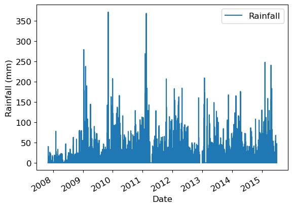
Lag-based features

train_df = rain_df.query("Date <= 20150630")
test_df = rain_df.query("Date >  20150630")

train_df.head()

	Date	Location	MinTemp	MaxTemp	Rainfall	Evaporation	Sunshine	WindGustDir	WindGustSpeed	WindDir9am	...	Humidity9am	Humidity3pm	Pressure9am	Pressure3pm	Cloud9am	Cloud3pm	Temp9am	Temp3pm	RainToday	RainTomorrow
0	2008-12-01	Albury	13.4	22.9	0.6	NaN	NaN	W	44.0	W	...	71.0	22.0	1007.7	1007.1	8.0	NaN	16.9	21.8	No	No
1	2008-12-02	Albury	7.4	25.1	0.0	NaN	NaN	WNW	44.0	NNW	...	44.0	25.0	1010.6	1007.8	NaN	NaN	17.2	24.3	No	No
2	2008-12-03	Albury	12.9	25.7	0.0	NaN	NaN	WSW	46.0	W	...	38.0	30.0	1007.6	1008.7	NaN	2.0	21.0	23.2	No	No
3	2008-12-04	Albury	9.2	28.0	0.0	NaN	NaN	NE	24.0	SE	...	45.0	16.0	1017.6	1012.8	NaN	NaN	18.1	26.5	No	No
4	2008-12-05	Albury	17.5	32.3	1.0	NaN	NaN	W	41.0	ENE	...	82.0	33.0	1010.8	1006.0	7.0	8.0	17.8	29.7	No	No

5 rows × 23 columns

• It looks like the dataframe is already sorted by Location and then by date for each Location.

• We could have done this ourselves with:

# train_df.sort_values(by=["Location", "Date"])

But make sure to also sort the targets (i.e. do this before preprocessing).

We can “lag” (or “shift”) a time series in Pandas with the .shift() method.

train_df = train_df.assign(Rainfall_lag1=train_df["Rainfall"].shift(1))

train_df[["Date", "Location", "Rainfall", "Rainfall_lag1"]][:20]

	Date	Location	Rainfall	Rainfall_lag1
0	2008-12-01	Albury	0.6	NaN
1	2008-12-02	Albury	0.0	0.6
2	2008-12-03	Albury	0.0	0.0
3	2008-12-04	Albury	0.0	0.0
4	2008-12-05	Albury	1.0	0.0
5	2008-12-06	Albury	0.2	1.0
6	2008-12-07	Albury	0.0	0.2
7	2008-12-08	Albury	0.0	0.0
8	2008-12-09	Albury	0.0	0.0
9	2008-12-10	Albury	1.4	0.0
10	2008-12-11	Albury	0.0	1.4
11	2008-12-12	Albury	2.2	0.0
12	2008-12-13	Albury	15.6	2.2
13	2008-12-14	Albury	3.6	15.6
15	2008-12-16	Albury	NaN	3.6
16	2008-12-17	Albury	0.0	NaN
17	2008-12-18	Albury	16.8	0.0
18	2008-12-19	Albury	10.6	16.8
19	2008-12-20	Albury	0.0	10.6
20	2008-12-21	Albury	0.0	0.0

• But we have multiple time series here and we need to be more careful with this.

• When we switch from one location to another we do not want to take the value from the previous location.

def create_lag_feature(df, orig_feature, lag):
    """Creates a new df with a new feature that's a lagged version of the original, where lag is an int."""
    # note: pandas .shift() kind of does this for you already, but oh well I already wrote this code

    new_df = df.copy()
    new_feature_name = "%s_lag%d" % (orig_feature, lag)
    new_df[new_feature_name] = np.nan
    for location, df_location in new_df.groupby(
        "Location"
    ):  # Each location is its own time series
        new_df.loc[df_location.index[lag:], new_feature_name] = df_location.iloc[:-lag][
            orig_feature
        ].values
    return new_df

train_df = create_lag_feature(train_df, "Rainfall", 1)

train_df[["Date", "Location", "Rainfall", "Rainfall_lag1"]][2285:2295]

	Date	Location	Rainfall	Rainfall_lag1
2309	2015-06-26	Albury	0.2	1.0
2310	2015-06-27	Albury	0.0	0.2
2311	2015-06-28	Albury	0.2	0.0
2312	2015-06-29	Albury	0.0	0.2
2313	2015-06-30	Albury	0.0	0.0
3040	2009-01-01	BadgerysCreek	0.0	NaN
3041	2009-01-02	BadgerysCreek	0.0	0.0
3042	2009-01-03	BadgerysCreek	0.0	0.0
3043	2009-01-04	BadgerysCreek	0.0	0.0
3044	2009-01-05	BadgerysCreek	0.0	0.0

Now it looks good!

• Question: is it OK to do this to the test set? Discuss.

• It’s fine if you would have this information available in deployment.

• If we’re just forecasting the next day, we should.

• Let’s include it for now.

rain_df_modified = create_lag_feature(rain_df, "Rainfall", 1)
train_df = rain_df_modified.query("Date <= 20150630")
test_df = rain_df_modified.query("Date >  20150630")

rain_df_modified

	Date	Location	MinTemp	MaxTemp	Rainfall	Evaporation	Sunshine	WindGustDir	WindGustSpeed	WindDir9am	...	Humidity3pm	Pressure9am	Pressure3pm	Cloud9am	Cloud3pm	Temp9am	Temp3pm	RainToday	RainTomorrow	Rainfall_lag1
0	2008-12-01	Albury	13.4	22.9	0.6	NaN	NaN	W	44.0	W	...	22.0	1007.7	1007.1	8.0	NaN	16.9	21.8	No	No	NaN
1	2008-12-02	Albury	7.4	25.1	0.0	NaN	NaN	WNW	44.0	NNW	...	25.0	1010.6	1007.8	NaN	NaN	17.2	24.3	No	No	0.6
2	2008-12-03	Albury	12.9	25.7	0.0	NaN	NaN	WSW	46.0	W	...	30.0	1007.6	1008.7	NaN	2.0	21.0	23.2	No	No	0.0
3	2008-12-04	Albury	9.2	28.0	0.0	NaN	NaN	NE	24.0	SE	...	16.0	1017.6	1012.8	NaN	NaN	18.1	26.5	No	No	0.0
4	2008-12-05	Albury	17.5	32.3	1.0	NaN	NaN	W	41.0	ENE	...	33.0	1010.8	1006.0	7.0	8.0	17.8	29.7	No	No	0.0
...	...	...	...	...	...	...	...	...	...	...	...	...	...	...	...	...	...	...	...	...	...
145454	2017-06-20	Uluru	3.5	21.8	0.0	NaN	NaN	E	31.0	ESE	...	27.0	1024.7	1021.2	NaN	NaN	9.4	20.9	No	No	0.0
145455	2017-06-21	Uluru	2.8	23.4	0.0	NaN	NaN	E	31.0	SE	...	24.0	1024.6	1020.3	NaN	NaN	10.1	22.4	No	No	0.0
145456	2017-06-22	Uluru	3.6	25.3	0.0	NaN	NaN	NNW	22.0	SE	...	21.0	1023.5	1019.1	NaN	NaN	10.9	24.5	No	No	0.0
145457	2017-06-23	Uluru	5.4	26.9	0.0	NaN	NaN	N	37.0	SE	...	24.0	1021.0	1016.8	NaN	NaN	12.5	26.1	No	No	0.0
145458	2017-06-24	Uluru	7.8	27.0	0.0	NaN	NaN	SE	28.0	SSE	...	24.0	1019.4	1016.5	3.0	2.0	15.1	26.0	No	No	0.0

142193 rows × 24 columns

X_train_enc, y_train, X_test_enc, y_test, preprocessor = preprocess_features(
    train_df,
    test_df,
    numeric_features + ["Rainfall_lag1"],
    categorical_features,
    drop_features,
    target
)

lr_coef = score_lr_print_coeff(
    preprocessor, train_df, y_train, test_df, y_test, X_train_enc
)

Train score: 0.85
Test score: 0.84

lr_coef.loc[["Rainfall", "Rainfall_lag1"]]

	Coef
Rainfall	0.081042
Rainfall_lag1	0.008300

• Rainfall from today has a positive coefficient.

• Rainfall from yesterday has a positive but a smaller coefficient.

• If we didn’t have rainfall from today feature, rainfall from yesterday feature would have received a bigger coefficient.

• We could also create a lagged version of the target.

• In fact, this dataset already has that built in! RainToday is the lagged version of the target RainTomorrow.

• We could also create lagged version of other features, or more lags

rain_df_modified = create_lag_feature(rain_df, "Rainfall", 1)
rain_df_modified = create_lag_feature(rain_df_modified, "Rainfall", 2)
rain_df_modified = create_lag_feature(rain_df_modified, "Rainfall", 3)
rain_df_modified = create_lag_feature(rain_df_modified, "Humidity3pm", 1)

rain_df_modified[
    [
        "Date",
        "Location",
        "Rainfall",
        "Rainfall_lag1",
        "Rainfall_lag2",
        "Rainfall_lag3",
        "Humidity3pm",
        "Humidity3pm_lag1",
    ]
].head(10)

	Date	Location	Rainfall	Rainfall_lag1	Rainfall_lag2	Rainfall_lag3	Humidity3pm	Humidity3pm_lag1
0	2008-12-01	Albury	0.6	NaN	NaN	NaN	22.0	NaN
1	2008-12-02	Albury	0.0	0.6	NaN	NaN	25.0	22.0
2	2008-12-03	Albury	0.0	0.0	0.6	NaN	30.0	25.0
3	2008-12-04	Albury	0.0	0.0	0.0	0.6	16.0	30.0
4	2008-12-05	Albury	1.0	0.0	0.0	0.0	33.0	16.0
5	2008-12-06	Albury	0.2	1.0	0.0	0.0	23.0	33.0
6	2008-12-07	Albury	0.0	0.2	1.0	0.0	19.0	23.0
7	2008-12-08	Albury	0.0	0.0	0.2	1.0	19.0	19.0
8	2008-12-09	Albury	0.0	0.0	0.0	0.2	9.0	19.0
9	2008-12-10	Albury	1.4	0.0	0.0	0.0	27.0	9.0

Note the pattern of NaN values.

train_df = rain_df_modified.query("Date <= 20150630")
test_df = rain_df_modified.query("Date >  20150630")

X_train_enc, y_train, X_test_enc, y_test, preprocessor = preprocess_features(
    train_df,
    test_df,
    numeric_features
    + ["Rainfall_lag1", "Rainfall_lag2", "Rainfall_lag3", "Humidity3pm_lag1"],
    categorical_features,
    drop_features,
    target
)

lr_coef = score_lr_print_coeff(
    preprocessor, train_df, y_train, test_df, y_test, X_train_enc
)

Train score: 0.85
Test score: 0.85

lr_coef.loc[
    [
        "Rainfall",
        "Rainfall_lag1",
        "Rainfall_lag2",
        "Rainfall_lag3",
        "Humidity3pm",
        "Humidity3pm_lag1",
    ]
]

	Coef
Rainfall	0.108487
Rainfall_lag1	0.023054
Rainfall_lag2	0.018269
Rainfall_lag3	0.017801
Humidity3pm	1.278574
Humidity3pm_lag1	-0.267491

Note the pattern in the magnitude of the coefficients.

Final remarks

What did we not cover?

• A huge amount!

Traditional time series approaches

• Time series analysis is a huge field of its own

• Traditional approaches include the ARIMA model and its various components/extensions.

• In Python, the statsmodels package is the place to go for this sort of thing.

  • For example, statsmodels.tsa.arima_model.ARIMA.

• These approaches can forecast, but they are also very good for understanding the temporal relationships in your data.

• We took different route in this course, and stick to our supervised learning tools.

Deep learning

• Recently, deep learning has been very successful too.

• In particular, recurrent neural networks (RNNs).

  • These are not covered in CPSC 340, but I believe they are in 540 (soon to be renamed 440).

  • LSTMs especially have shown a lot of promise in this type of task.

  • Here is a blog post about LSTMs.

Types of problems involving time series

• A single label associated with an entire time series.

  • We had that with images earlier on, you could have the same for a time series.

  • E.g., for fraud detection, labelling each transaction as fraud/normal vs. labelling a person as bad/good based on their entire history.

  • There are various approaches that can be used for this type of problem, including CNNs (Lecture 19), LSTMs, and non deep learning methods.

• Inference problems

  • What are the patterns in this time series?

  • How many lags are associated with the current value?

  • Etc.

Unequally spaced time points

• We assumed we have a measurement each day.

• For example, when creating lag features we used consecutive rows in the DataFrame.

• But, in fact some days were missing in this dataset.

• More generally, what if the measurements are at arbitrary times, not equally spaced?

  • Some of our approaches would still work, like encoding the month.

  • Some of our approaches would not make sense, like the lags.

  • Perhaps the measurements could be binned into equally spaced bins, or something.

  • This is more of a hassle.

Other software package

• A good one to know about is Prophet.

• sktime

  • Time series classification

  • forecasting

• tslearn

  • classification

  • regression

  • clustering

Feature engineering

• Often, a useful approach is to just engineer your own features.

  • E.g., max expenditure, min expenditure, max-min, avg time gap between transactions, variance of time gap between transactions, etc etc.

  • We could do that here as well, or in any problem.