Lecture 15: Class demo#
Let’s cluster images!!
For this demo, I’m going to use the following image dataset:
A tiny subset of Food-101 from last lecture (available here).
A small subset of Human Faces dataset (available here).
To run the code below, you need to install pytorch and torchvision in the course conda environment.
conda install pytorch torchvision -c pytorch
import os, sys
sys.path.append(os.path.join(os.path.abspath(".."), "code"))
from plotting_functions_unsup import *
import random
import numpy as np
import pandas as pd
import torch
from torchvision import datasets, models, transforms, utils
from PIL import Image
from torchvision import transforms
from torchvision.models import vgg16
import matplotlib.pyplot as plt
import torchvision
Let’s start with small subset of birds dataset. You can experiment with a bigger dataset if you like.
device = torch.device("cuda:0" if torch.cuda.is_available() else "cpu")
def set_seed(seed=42):
    torch.manual_seed(seed)
    np.random.seed(seed)
    random.seed(seed)
set_seed(seed=42)
import glob
IMAGE_SIZE = 200
def read_img_dataset(data_dir):
    data_transforms = transforms.Compose(
        [
            transforms.Resize((IMAGE_SIZE, IMAGE_SIZE)),
            transforms.ToTensor(),
            transforms.Normalize([0.5, 0.5, 0.5], [0.5, 0.5, 0.5]),
        ])

    image_dataset = datasets.ImageFolder(root=data_dir, transform=data_transforms)
    dataloader = torch.utils.data.DataLoader(
         image_dataset, batch_size=BATCH_SIZE, shuffle=True, num_workers=0
    )
    dataset_size = len(image_dataset)
    class_names = image_dataset.classes
    inputs, classes = next(iter(dataloader))
    return inputs, classes
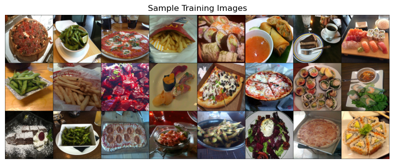
def plot_sample_imgs(inputs):
    plt.figure(figsize=(10, 70)); plt.axis("off"); plt.title("Sample Training Images")
    plt.imshow(np.transpose(utils.make_grid(inputs, padding=1, normalize=True),(1, 2, 0)));
def get_features(model, inputs):
    """Extract output of densenet model"""
    with torch.no_grad():  # turn off computational graph stuff
        Z_train = torch.empty((0, 1024))  # Initialize empty tensors
        y_train = torch.empty((0))
        Z_train = torch.cat((Z_train, model(inputs)), dim=0)
    return Z_train.detach()
densenet = models.densenet121(weights="DenseNet121_Weights.IMAGENET1K_V1")
densenet.classifier = torch.nn.Identity()  # remove that last "classification" layer
data_dir = "../data/food"
file_names = [image_file for image_file in glob.glob(data_dir + "/*/*.jpg")]
n_images = len(file_names)
BATCH_SIZE = n_images  # because our dataset is quite small
food_inputs, food_classes = read_img_dataset(data_dir)
n_images
350
X_food = food_inputs.numpy()
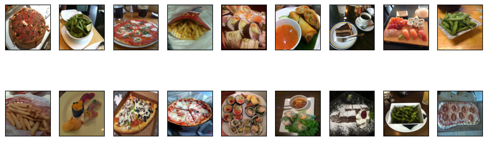
plot_sample_imgs(food_inputs[0:24,:,:,:])
Z_food = get_features(
    densenet, food_inputs,
)
Z_food = Z_food.numpy()
Z_food.shape
(350, 1024)
from sklearn.cluster import KMeans

k = 7
km = KMeans(n_clusters=k, n_init='auto', random_state=123)
km.fit(Z_food)
KMeans(n_clusters=7, n_init='auto', random_state=123)In a Jupyter environment, please rerun this cell to show the HTML representation or trust the notebook.
On GitHub, the HTML representation is unable to render, please try loading this page with nbviewer.org.
KMeans(n_clusters=7, n_init='auto', random_state=123)
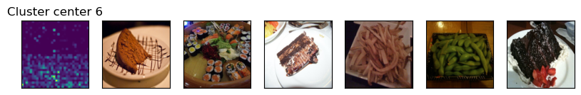
for cluster in range(k):
    get_cluster_images(km, Z_food, X_food, cluster, n_img=6)
Image indices: [ 82 58 168 114 122 44]
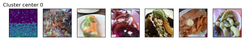
Image indices: [ 89 209 67 330 141 166]
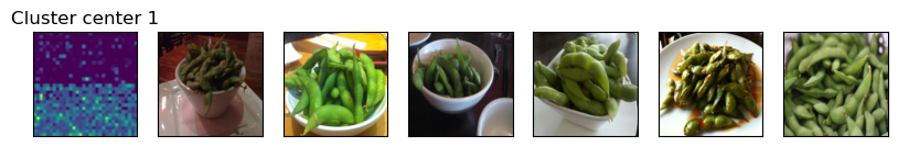
Image indices: [249 327 331 30 236 267]
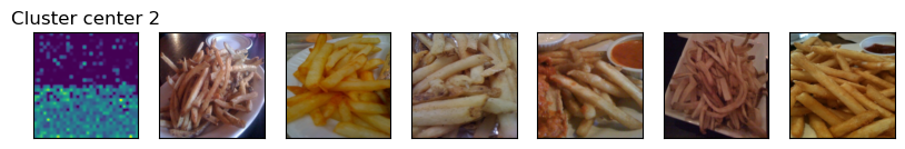
Image indices: [ 76 90 29 240 237 238]
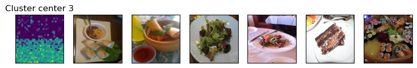
Image indices: [223 136 124 304 13 137]
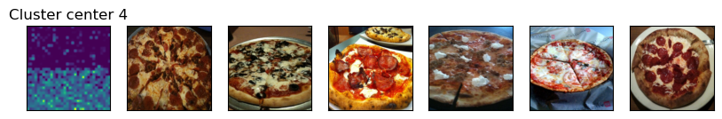
Image indices: [190 132 73 140 6 149]
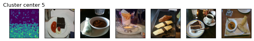
Image indices: [ 65 238 237 236 235 234]
Let’s try DBSCAN.
dbscan = DBSCAN()

labels = dbscan.fit_predict(Z_food)
print("Unique labels: {}".format(np.unique(labels)))
Unique labels: [-1]
It identified all points as noise points. Let’s explore the distances between points.
from sklearn.metrics.pairwise import euclidean_distances

dists = euclidean_distances(Z_food)
np.fill_diagonal(dists, np.inf)
dists_df = pd.DataFrame(dists)
dists_df
| 0 | 1 | 2 | 3 | 4 | 5 | 6 | 7 | 8 | 9 | ... | 340 | 341 | 342 | 343 | 344 | 345 | 346 | 347 | 348 | 349 | |
|---|---|---|---|---|---|---|---|---|---|---|---|---|---|---|---|---|---|---|---|---|---|
| 0 | inf | 27.838209 | 24.272423 | 28.557386 | 25.911512 | 26.729088 | 28.535007 | 27.919943 | 29.910038 | 24.831701 | ... | 25.821581 | 27.069433 | 27.836058 | 27.045502 | 28.334972 | 28.312830 | 30.730888 | 26.483530 | 26.518341 | 27.012949 |
| 1 | 27.838209 | inf | 25.690664 | 26.808674 | 28.380119 | 26.499969 | 25.269186 | 27.080601 | 24.174231 | 26.724173 | ... | 25.517481 | 22.425566 | 24.153849 | 26.348946 | 28.451920 | 27.344963 | 26.383554 | 24.948429 | 23.117655 | 25.012907 |
| 2 | 24.272423 | 25.690664 | inf | 26.241850 | 26.272598 | 24.983030 | 25.745886 | 26.138418 | 27.259501 | 23.387449 | ... | 24.976543 | 24.755798 | 26.489601 | 26.757547 | 23.980059 | 25.965456 | 29.195887 | 25.397800 | 23.607014 | 23.029932 |
| 3 | 28.557386 | 26.808674 | 26.241850 | inf | 28.488819 | 26.426289 | 28.817778 | 29.362293 | 27.543203 | 22.214371 | ... | 24.433807 | 26.525894 | 26.772890 | 28.805965 | 26.740297 | 24.505461 | 29.599627 | 27.887571 | 26.735687 | 26.722355 |
| 4 | 25.911512 | 28.380119 | 26.272598 | 28.488819 | inf | 25.054052 | 28.763035 | 28.249685 | 29.294979 | 24.665562 | ... | 25.088818 | 26.409763 | 27.046513 | 26.512915 | 28.122980 | 26.731318 | 29.328199 | 26.524778 | 26.566645 | 26.233059 |
| ... | ... | ... | ... | ... | ... | ... | ... | ... | ... | ... | ... | ... | ... | ... | ... | ... | ... | ... | ... | ... | ... |
| 345 | 28.312830 | 27.344963 | 25.965456 | 24.505461 | 26.731318 | 27.732960 | 28.961937 | 28.021688 | 28.355204 | 24.388792 | ... | 23.226387 | 25.771818 | 26.816877 | 29.633665 | 27.816105 | inf | 29.698130 | 26.911955 | 25.400141 | 26.690134 |
| 346 | 30.730888 | 26.383554 | 29.195887 | 29.599627 | 29.328199 | 27.754042 | 30.597506 | 31.449287 | 29.049765 | 26.228279 | ... | 26.203318 | 26.634016 | 25.843769 | 28.824900 | 31.539536 | 29.698130 | inf | 28.891027 | 29.559868 | 28.736403 |
| 347 | 26.483530 | 24.948429 | 25.397800 | 27.887571 | 26.524778 | 25.069878 | 26.720396 | 27.640726 | 28.087231 | 24.709068 | ... | 24.990519 | 25.950739 | 26.422796 | 23.982191 | 27.307524 | 26.911955 | 28.891027 | inf | 24.929638 | 22.822123 |
| 348 | 26.518341 | 23.117655 | 23.607014 | 26.735687 | 26.566645 | 23.524864 | 23.816399 | 25.144579 | 25.315739 | 25.252844 | ... | 25.219345 | 23.628778 | 24.586554 | 24.797318 | 25.021420 | 25.400141 | 29.559868 | 24.929638 | inf | 24.156252 |
| 349 | 27.012949 | 25.012907 | 23.029932 | 26.722355 | 26.233059 | 25.000036 | 24.752766 | 26.942122 | 27.648315 | 25.040714 | ... | 24.330954 | 25.934887 | 26.133183 | 24.376286 | 26.258141 | 26.690134 | 28.736403 | 22.822123 | 24.156252 | inf |
350 rows × 350 columns
dists.min(), np.nanmax(dists[dists != np.inf]), np.mean(dists[dists != np.inf])
(14.918853, 39.791836, 27.870182)
for eps in range(16, 30):
    print("\neps={}".format(eps))
    dbscan = DBSCAN(eps=eps, min_samples=3)
    labels = dbscan.fit_predict(Z_food)
    print("Number of clusters: {}".format(len(np.unique(labels))))
    print("Cluster sizes: {}".format(np.bincount(labels + 1)))
eps=16
Number of clusters: 1
Cluster sizes: [350]

eps=17
Number of clusters: 3
Cluster sizes: [341   5   4]

eps=18
Number of clusters: 3
Cluster sizes: [334  13   3]

eps=19
Number of clusters: 3
Cluster sizes: [311  35   4]

eps=20
Number of clusters: 4
Cluster sizes: [274  70   3   3]

eps=21
Number of clusters: 2
Cluster sizes: [234 116]

eps=22
Number of clusters: 2
Cluster sizes: [182 168]

eps=23
Number of clusters: 2
Cluster sizes: [132 218]

eps=24
Number of clusters: 2
Cluster sizes: [ 81 269]

eps=25
Number of clusters: 2
Cluster sizes: [ 52 298]

eps=26
Number of clusters: 2
Cluster sizes: [ 30 320]

eps=27
Number of clusters: 2
Cluster sizes: [ 17 333]

eps=28
Number of clusters: 2
Cluster sizes: [  5 345]

eps=29
Number of clusters: 2
Cluster sizes: [  2 348]
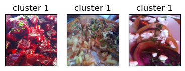
dbscan = DBSCAN(eps=18, min_samples=3)
dbscan_labels = dbscan.fit_predict(Z_food)
print("Number of clusters: {}".format(len(np.unique(dbscan_labels))))
print("Cluster sizes: {}".format(np.bincount(dbscan_labels + 1)))
print("Unique labels: {}".format(np.unique(dbscan_labels)))
Number of clusters: 3
Cluster sizes: [334  13   3]
Unique labels: [-1  0  1]
print_dbscan_clusters(Z_food, food_inputs, dbscan_labels)

Let’s examine noise points identified by DBSCAN.
print_dbscan_noise_images(Z_food, food_inputs, dbscan_labels)
Now let’s try another dataset with human faces, a small subset of Human Faces dataset (available here).
data_dir = "../data/test"
file_names = [image_file for image_file in glob.glob(data_dir + "/*/*.jpg")]
n_images = len(file_names)
BATCH_SIZE = n_images  # because our dataset is quite small
faces_inputs, classes = read_img_dataset(data_dir)
X_faces = faces_inputs.numpy()
X_faces.shape
(367, 3, 200, 200)
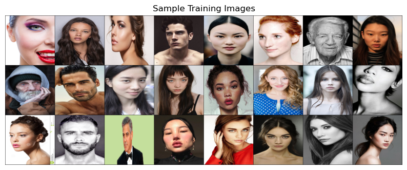
plot_sample_imgs(faces_inputs[0:24,:,:,:])
Z_faces = get_features(
    densenet, faces_inputs,
).numpy()
Z_faces.shape
(367, 1024)
from sklearn.cluster import KMeans

k = 7
km = KMeans(n_clusters=k, n_init='auto', random_state=123)
km.fit(Z_faces)
KMeans(n_clusters=7, n_init='auto', random_state=123)In a Jupyter environment, please rerun this cell to show the HTML representation or trust the notebook.
On GitHub, the HTML representation is unable to render, please try loading this page with nbviewer.org.
KMeans(n_clusters=7, n_init='auto', random_state=123)
km.cluster_centers_.shape
(7, 1024)
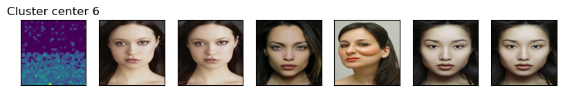
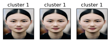
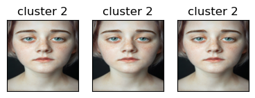
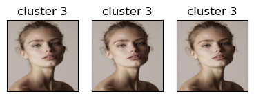
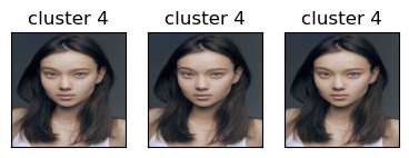
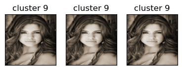
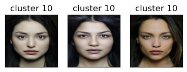
for cluster in range(k):
    get_cluster_images(km, Z_faces, X_faces, cluster, n_img=6)
Image indices: [136 175 355 285 56 346]
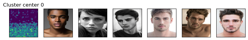
Image indices: [117 320 208 216 186 59]
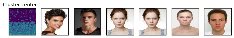
Image indices: [103 353 359 295 68 60]
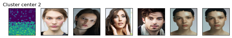
Image indices: [ 39 357 332 256 218 1]
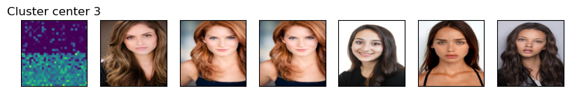
Image indices: [317 168 267 0 248 247]
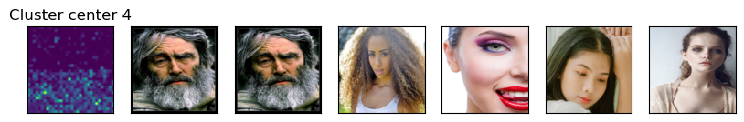
Image indices: [290 124 271 83 139 146]
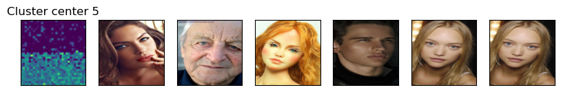
Image indices: [312 260 329 127 40 348]
Clustering faces with DBSCAN#
dbscan = DBSCAN()
labels = dbscan.fit_predict(Z_faces)
print("Unique labels: {}".format(np.unique(labels)))
Unique labels: [-1]
dists = euclidean_distances(Z_faces)
np.fill_diagonal(dists, np.inf)

dist_df = pd.DataFrame(
    dists
)

dist_df.iloc[10:20, 10:20]
| 10 | 11 | 12 | 13 | 14 | 15 | 16 | 17 | 18 | 19 | |
|---|---|---|---|---|---|---|---|---|---|---|
| 10 | inf | 22.212444 | 29.023613 | 24.863905 | 22.001663 | 24.938940 | 28.098724 | 30.955692 | 27.270945 | 27.389570 |
| 11 | 22.212444 | inf | 27.826571 | 22.514793 | 19.561979 | 26.348663 | 26.740641 | 31.028826 | 27.770222 | 27.892704 |
| 12 | 29.023613 | 27.826571 | inf | 27.719786 | 28.463976 | 27.759411 | 26.995085 | 29.543497 | 29.854399 | 25.650290 |
| 13 | 24.863905 | 22.514793 | 27.719786 | inf | 22.240793 | 24.963823 | 25.705948 | 29.509878 | 27.242216 | 26.694988 |
| 14 | 22.001663 | 19.561979 | 28.463976 | 22.240793 | inf | 25.906570 | 27.872011 | 29.647667 | 28.404259 | 27.862476 |
| 15 | 24.938940 | 26.348663 | 27.759411 | 24.963823 | 25.906570 | inf | 27.595673 | 26.784702 | 28.887432 | 25.958988 |
| 16 | 28.098724 | 26.740641 | 26.995085 | 25.705948 | 27.872011 | 27.595673 | inf | 29.354176 | 28.925968 | 26.882242 |
| 17 | 30.955692 | 31.028826 | 29.543497 | 29.509878 | 29.647667 | 26.784702 | 29.354176 | inf | 33.242348 | 29.911688 |
| 18 | 27.270945 | 27.770222 | 29.854399 | 27.242216 | 28.404259 | 28.887432 | 28.925968 | 33.242348 | inf | 29.257753 |
| 19 | 27.389570 | 27.892704 | 25.650290 | 26.694988 | 27.862476 | 25.958988 | 26.882242 | 29.911688 | 29.257753 | inf |
dists.min(), np.nanmax(dists[dists != np.inf]), np.mean(dists[dists != np.inf])
(0.0, 36.27959, 25.94334)
for eps in [16, 17, 18, 19, 20, 21, 22, 24]:
    print("\neps={}".format(eps))
    dbscan = DBSCAN(eps=eps, min_samples=3)
    labels = dbscan.fit_predict(Z_faces)
    print("Number of clusters: {}".format(len(np.unique(labels))))
    print("Cluster sizes: {}".format(np.bincount(labels + 1)))
eps=16
Number of clusters: 8
Cluster sizes: [345   3   3   3   3   4   3   3]

eps=17
Number of clusters: 12
Cluster sizes: [325   4   3   3   3   3   6   7   4   3   3   3]

eps=18
Number of clusters: 10
Cluster sizes: [305  33   3   3   3   7   3   4   3   3]

eps=19
Number of clusters: 9
Cluster sizes: [261  84   3   3   3   4   3   3   3]

eps=20
Number of clusters: 7
Cluster sizes: [211 140   3   4   3   3   3]

eps=21
Number of clusters: 5
Cluster sizes: [159 197   3   5   3]

eps=22
Number of clusters: 4
Cluster sizes: [100 261   3   3]

eps=24
Number of clusters: 2
Cluster sizes: [ 25 342]
dbscan = DBSCAN(eps=17, min_samples=3)
dbscan_labels = dbscan.fit_predict(Z_faces)
print("Number of clusters: {}".format(len(np.unique(dbscan_labels))))
print("Cluster sizes: {}".format(np.bincount(dbscan_labels + 1)))
print("Unique labels: {}".format(np.unique(dbscan_labels)))
Number of clusters: 12
Cluster sizes: [325   4   3   3   3   3   6   7   4   3   3   3]
Unique labels: [-1  0  1  2  3  4  5  6  7  8  9 10]
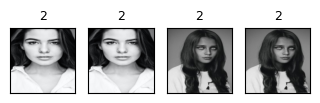
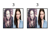
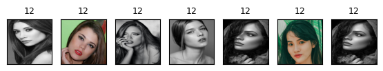
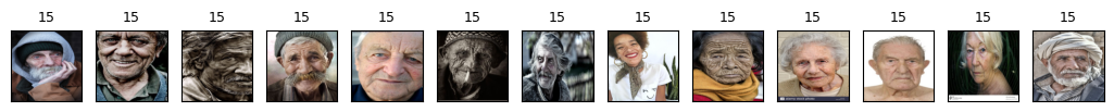
print_dbscan_clusters(Z_faces, faces_inputs, dbscan_labels)
Let’s examine noise images identified by DBSCAN.
print_dbscan_noise_images(Z_faces, faces_inputs, dbscan_labels)
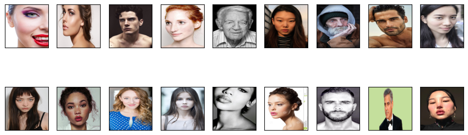
We can guess why these images are noise images. There are odd angles, cropping, sun glasses, hands near faces etc.
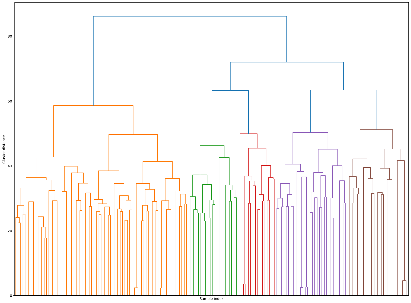
Hierarchical clustering#
set_seed(seed=42)
plt.figure(figsize=(20, 15))
Z_hrch = ward(Z_faces)
dendrogram(Z_hrch, p=7, truncate_mode="level", no_labels=True)
plt.xlabel("Sample index")
plt.ylabel("Cluster distance");
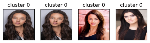
cluster_labels = fcluster(Z_hrch, 30, criterion="maxclust") # let's get flat clusters
#hand_picked_clusters = np.arange(2, 30)
hand_picked_clusters = [2, 3, 5, 6,7, 8, 9, 10, 12, 14,15,16,17,19,20, 21,22, 24, 26, 27, 28]
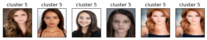
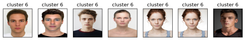
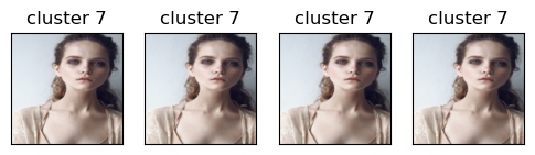
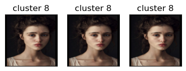
print_hierarchical_clusters(
faces_inputs, Z_faces, cluster_labels, hand_picked_clusters
)
/Users/kvarada/CS/2023-24/330/cpsc330-2023W1/lectures/code/plotting_functions_unsup.py:1490: RuntimeWarning:

More than 20 figures have been opened. Figures created through the pyplot interface (`matplotlib.pyplot.figure`) are retained until explicitly closed and may consume too much memory. (To control this warning, see the rcParam `figure.max_open_warning`). Consider using `matplotlib.pyplot.close()`.
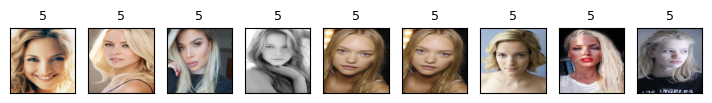


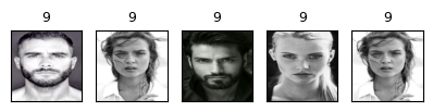


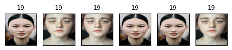
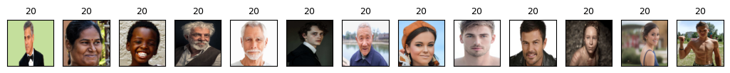

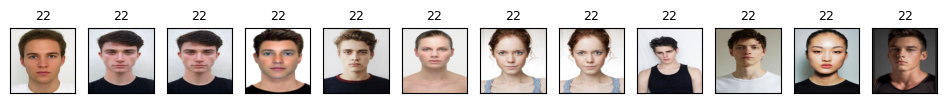

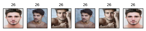
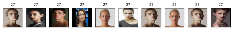
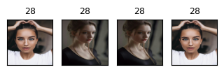
Some clusters correspond to people with distinct faces, age, facial expressions, hair colour and hair style, lighting and skin tone.