
Lecture 10: Regression metrics#
UBC, 2023-24
Instructor: Varada Kolhatkar and Andrew Roth
Imports#
import matplotlib.pyplot as plt
import numpy as np
import pandas as pd
from sklearn.compose import (
    ColumnTransformer,
    TransformedTargetRegressor,
    make_column_transformer,
)
from sklearn.dummy import DummyRegressor
from sklearn.ensemble import RandomForestRegressor
from sklearn.impute import SimpleImputer
from sklearn.linear_model import Ridge, RidgeCV
from sklearn.metrics import make_scorer, mean_squared_error, r2_score
from sklearn.model_selection import (
    GridSearchCV,
    cross_val_score,
    cross_validate,
    train_test_split,
)
from sklearn.pipeline import Pipeline, make_pipeline
from sklearn.preprocessing import OneHotEncoder, OrdinalEncoder, StandardScaler
from sklearn.tree import DecisionTreeRegressor

%matplotlib inline
import warnings

warnings.simplefilter(action="ignore", category=FutureWarning)
Announcements#
HW4 is due tonight.
HW5 will be posted today. It is a project-type homework assignment and will be due after the midterm.
Midterm: Thursday, October 26th, 2023 at 6:00pm (~75 mins long)
Checkout the midterm information announcement on Piazza (@407)
Learning outcomes#
From this lecture, students are expected to be able to:
Carry out feature transformations on somewhat complicated dataset.
Visualize transformed features as a dataframe.
Use
RidgeandRidgeCV.Explain how
alphahyperparameter ofRidgerelates to the fundamental tradeoff.Explain the effect of
alphaon the magnitude of the learned coefficients.Examine coefficients of transformed features.
Appropriately select a scoring metric given a regression problem.
Interpret and communicate the meanings of different scoring metrics on regression problems.
MSE, RMSE, \(R^2\), MAPE
Apply log-transform on the target values in a regression problem with
TransformedTargetRegressor.
After carrying out preprocessing, why it’s useful to get feature names for transformed features?
More comments on tackling class imbalance#
In lecture 9 we talked about a few rather simple approaches to deal with class imbalance.
If you have a problem such as fraud detection problem where you want to spot rare events, you can also think of this problem as anomaly detection problem and use different kinds of algorithms such as isolation forests.
If you are interested in this area, it might be worth checking out this book on this topic. Imbalanced Learning: Foundations, Algorithms, and Applications
Note
When you calculate precision, recall, f1 score, by default only the positive label is evaluated, assuming by default that the positive class is labeled 1. This is configurable through the pos_label parameter.
Dataset [video]#
In this lecture, we’ll be using Kaggle House Prices dataset. As usual, to run this notebook you’ll need to download the data. For this dataset, train and test have already been separated. We’ll be working with the train portion in this lecture.
df = pd.read_csv("data/housing-kaggle/train.csv")
train_df, test_df = train_test_split(df, test_size=0.10, random_state=123)
train_df.head()
| Id | MSSubClass | MSZoning | LotFrontage | LotArea | Street | Alley | LotShape | LandContour | Utilities | ... | PoolArea | PoolQC | Fence | MiscFeature | MiscVal | MoSold | YrSold | SaleType | SaleCondition | SalePrice | |
|---|---|---|---|---|---|---|---|---|---|---|---|---|---|---|---|---|---|---|---|---|---|
| 302 | 303 | 20 | RL | 118.0 | 13704 | Pave | NaN | IR1 | Lvl | AllPub | ... | 0 | NaN | NaN | NaN | 0 | 1 | 2006 | WD | Normal | 205000 |
| 767 | 768 | 50 | RL | 75.0 | 12508 | Pave | NaN | IR1 | Lvl | AllPub | ... | 0 | NaN | NaN | Shed | 1300 | 7 | 2008 | WD | Normal | 160000 |
| 429 | 430 | 20 | RL | 130.0 | 11457 | Pave | NaN | IR1 | Lvl | AllPub | ... | 0 | NaN | NaN | NaN | 0 | 3 | 2009 | WD | Normal | 175000 |
| 1139 | 1140 | 30 | RL | 98.0 | 8731 | Pave | NaN | IR1 | Lvl | AllPub | ... | 0 | NaN | NaN | NaN | 0 | 5 | 2007 | WD | Normal | 144000 |
| 558 | 559 | 60 | RL | 57.0 | 21872 | Pave | NaN | IR2 | HLS | AllPub | ... | 0 | NaN | NaN | NaN | 0 | 8 | 2008 | WD | Normal | 175000 |
5 rows × 81 columns
The supervised machine learning problem is predicting housing price given features associated with properties.
Here, the target is
SalePrice, which is continuous. So it’s a regression problem (as opposed to classification).
train_df.shape
(1314, 81)
Let’s separate X and y#
X_train = train_df.drop(columns=["SalePrice"])
y_train = train_df["SalePrice"]

X_test = test_df.drop(columns=["SalePrice"])
y_test = test_df["SalePrice"]
EDA#
train_df.describe()
| Id | MSSubClass | LotFrontage | LotArea | OverallQual | OverallCond | YearBuilt | YearRemodAdd | MasVnrArea | BsmtFinSF1 | ... | WoodDeckSF | OpenPorchSF | EnclosedPorch | 3SsnPorch | ScreenPorch | PoolArea | MiscVal | MoSold | YrSold | SalePrice | |
|---|---|---|---|---|---|---|---|---|---|---|---|---|---|---|---|---|---|---|---|---|---|
| count | 1314.000000 | 1314.000000 | 1089.000000 | 1314.000000 | 1314.000000 | 1314.000000 | 1314.000000 | 1314.000000 | 1307.000000 | 1314.000000 | ... | 1314.000000 | 1314.000000 | 1314.000000 | 1314.000000 | 1314.000000 | 1314.000000 | 1314.000000 | 1314.000000 | 1314.000000 | 1314.000000 |
| mean | 734.182648 | 56.472603 | 69.641873 | 10273.261035 | 6.076104 | 5.570015 | 1970.995434 | 1984.659056 | 102.514155 | 441.425419 | ... | 94.281583 | 45.765601 | 21.726788 | 3.624049 | 13.987062 | 3.065449 | 46.951294 | 6.302131 | 2007.840183 | 179802.147641 |
| std | 422.224662 | 42.036646 | 23.031794 | 8997.895541 | 1.392612 | 1.112848 | 30.198127 | 20.639754 | 178.301563 | 459.276687 | ... | 125.436492 | 65.757545 | 60.766423 | 30.320430 | 53.854129 | 42.341109 | 522.283421 | 2.698206 | 1.332824 | 79041.260572 |
| min | 1.000000 | 20.000000 | 21.000000 | 1300.000000 | 1.000000 | 1.000000 | 1872.000000 | 1950.000000 | 0.000000 | 0.000000 | ... | 0.000000 | 0.000000 | 0.000000 | 0.000000 | 0.000000 | 0.000000 | 0.000000 | 1.000000 | 2006.000000 | 34900.000000 |
| 25% | 369.250000 | 20.000000 | 59.000000 | 7500.000000 | 5.000000 | 5.000000 | 1953.000000 | 1966.250000 | 0.000000 | 0.000000 | ... | 0.000000 | 0.000000 | 0.000000 | 0.000000 | 0.000000 | 0.000000 | 0.000000 | 5.000000 | 2007.000000 | 129600.000000 |
| 50% | 735.500000 | 50.000000 | 69.000000 | 9391.000000 | 6.000000 | 5.000000 | 1972.000000 | 1993.000000 | 0.000000 | 376.000000 | ... | 0.000000 | 24.000000 | 0.000000 | 0.000000 | 0.000000 | 0.000000 | 0.000000 | 6.000000 | 2008.000000 | 162000.000000 |
| 75% | 1099.750000 | 70.000000 | 80.000000 | 11509.000000 | 7.000000 | 6.000000 | 2000.000000 | 2004.000000 | 165.500000 | 704.750000 | ... | 168.000000 | 66.750000 | 0.000000 | 0.000000 | 0.000000 | 0.000000 | 0.000000 | 8.000000 | 2009.000000 | 212975.000000 |
| max | 1460.000000 | 190.000000 | 313.000000 | 215245.000000 | 10.000000 | 9.000000 | 2010.000000 | 2010.000000 | 1378.000000 | 5644.000000 | ... | 857.000000 | 547.000000 | 552.000000 | 508.000000 | 480.000000 | 738.000000 | 15500.000000 | 12.000000 | 2010.000000 | 755000.000000 |
8 rows × 38 columns
train_df.info()
<class 'pandas.core.frame.DataFrame'>
Index: 1314 entries, 302 to 1389
Data columns (total 81 columns):
 #   Column         Non-Null Count  Dtype
---  ------         --------------  -----
 0   Id             1314 non-null   int64
 1   MSSubClass     1314 non-null   int64
 2   MSZoning       1314 non-null   object
 3   LotFrontage    1089 non-null   float64
 4   LotArea        1314 non-null   int64
 5   Street         1314 non-null   object
 6   Alley          81 non-null     object
 7   LotShape       1314 non-null   object
 8   LandContour    1314 non-null   object
 9   Utilities      1314 non-null   object
 10  LotConfig      1314 non-null   object
 11  LandSlope      1314 non-null   object
 12  Neighborhood   1314 non-null   object
 13  Condition1     1314 non-null   object
 14  Condition2     1314 non-null   object
 15  BldgType       1314 non-null   object
 16  HouseStyle     1314 non-null   object
 17  OverallQual    1314 non-null   int64
 18  OverallCond    1314 non-null   int64
 19  YearBuilt      1314 non-null   int64
 20  YearRemodAdd   1314 non-null   int64
 21  RoofStyle      1314 non-null   object
 22  RoofMatl       1314 non-null   object
 23  Exterior1st    1314 non-null   object
 24  Exterior2nd    1314 non-null   object
 25  MasVnrType     528 non-null    object
 26  MasVnrArea     1307 non-null   float64
 27  ExterQual      1314 non-null   object
 28  ExterCond      1314 non-null   object
 29  Foundation     1314 non-null   object
 30  BsmtQual       1280 non-null   object
 31  BsmtCond       1280 non-null   object
 32  BsmtExposure   1279 non-null   object
 33  BsmtFinType1   1280 non-null   object
 34  BsmtFinSF1     1314 non-null   int64
 35  BsmtFinType2   1280 non-null   object
 36  BsmtFinSF2     1314 non-null   int64
 37  BsmtUnfSF      1314 non-null   int64
 38  TotalBsmtSF    1314 non-null   int64
 39  Heating        1314 non-null   object
 40  HeatingQC      1314 non-null   object
 41  CentralAir     1314 non-null   object
 42  Electrical     1313 non-null   object
 43  1stFlrSF       1314 non-null   int64
 44  2ndFlrSF       1314 non-null   int64
 45  LowQualFinSF   1314 non-null   int64
 46  GrLivArea      1314 non-null   int64
 47  BsmtFullBath   1314 non-null   int64
 48  BsmtHalfBath   1314 non-null   int64
 49  FullBath       1314 non-null   int64
 50  HalfBath       1314 non-null   int64
 51  BedroomAbvGr   1314 non-null   int64
 52  KitchenAbvGr   1314 non-null   int64
 53  KitchenQual    1314 non-null   object
 54  TotRmsAbvGrd   1314 non-null   int64
 55  Functional     1314 non-null   object
 56  Fireplaces     1314 non-null   int64
 57  FireplaceQu    687 non-null    object
 58  GarageType     1241 non-null   object
 59  GarageYrBlt    1241 non-null   float64
 60  GarageFinish   1241 non-null   object
 61  GarageCars     1314 non-null   int64
 62  GarageArea     1314 non-null   int64
 63  GarageQual     1241 non-null   object
 64  GarageCond     1241 non-null   object
 65  PavedDrive     1314 non-null   object
 66  WoodDeckSF     1314 non-null   int64
 67  OpenPorchSF    1314 non-null   int64
 68  EnclosedPorch  1314 non-null   int64
 69  3SsnPorch      1314 non-null   int64
 70  ScreenPorch    1314 non-null   int64
 71  PoolArea       1314 non-null   int64
 72  PoolQC         7 non-null      object
 73  Fence          259 non-null    object
 74  MiscFeature    50 non-null     object
 75  MiscVal        1314 non-null   int64
 76  MoSold         1314 non-null   int64
 77  YrSold         1314 non-null   int64
 78  SaleType       1314 non-null   object
 79  SaleCondition  1314 non-null   object
 80  SalePrice      1314 non-null   int64
dtypes: float64(3), int64(35), object(43)
memory usage: 841.8+ KB
pandas_profiler#
We do not have pandas_profiling in our course environment. You will have to install it in the environment on your own if you want to run the code below.
conda install -c conda-forge pandas-profiling
# from pandas_profiling import ProfileReport

# profile = ProfileReport(train_df, title="Pandas Profiling Report")  # , minimal=True)
# profile.to_notebook_iframe()
Feature types#
Do not blindly trust all the info given to you by automated tools.
How does pandas profiling figure out the data type?
You can look at the Python data type and say floats are numeric, strings are categorical.
However, in doing so you would miss out on various subtleties such as some of the string features being ordinal rather than truly categorical.
Also, it will think free text is categorical.
In addition to tools such as above, it’s important to go through data description to understand the data.
The data description for our dataset is available here.
Feature types#
We have mixed feature types and a bunch of missing values.
Now, let’s identify feature types and transformations.
Let’s get the numeric-looking columns.
numeric_looking_columns = X_train.select_dtypes(include=np.number).columns.tolist()
print(numeric_looking_columns)
['Id', 'MSSubClass', 'LotFrontage', 'LotArea', 'OverallQual', 'OverallCond', 'YearBuilt', 'YearRemodAdd', 'MasVnrArea', 'BsmtFinSF1', 'BsmtFinSF2', 'BsmtUnfSF', 'TotalBsmtSF', '1stFlrSF', '2ndFlrSF', 'LowQualFinSF', 'GrLivArea', 'BsmtFullBath', 'BsmtHalfBath', 'FullBath', 'HalfBath', 'BedroomAbvGr', 'KitchenAbvGr', 'TotRmsAbvGrd', 'Fireplaces', 'GarageYrBlt', 'GarageCars', 'GarageArea', 'WoodDeckSF', 'OpenPorchSF', 'EnclosedPorch', '3SsnPorch', 'ScreenPorch', 'PoolArea', 'MiscVal', 'MoSold', 'YrSold']
Not all numeric looking columns are necessarily numeric.
train_df["MSSubClass"].unique()
array([ 20,  50,  30,  60, 160,  85,  90, 120, 180,  80,  70,  75, 190,
        45,  40])
MSSubClass: Identifies the type of dwelling involved in the sale.
    20	1-STORY 1946 & NEWER ALL STYLES
    30	1-STORY 1945 & OLDER
    40	1-STORY W/FINISHED ATTIC ALL AGES
    45	1-1/2 STORY - UNFINISHED ALL AGES
    50	1-1/2 STORY FINISHED ALL AGES
    60	2-STORY 1946 & NEWER
    70	2-STORY 1945 & OLDER
    75	2-1/2 STORY ALL AGES
    80	SPLIT OR MULTI-LEVEL
    85	SPLIT FOYER
    90	DUPLEX - ALL STYLES AND AGES
   120	1-STORY PUD (Planned Unit Development) - 1946 & NEWER
   150	1-1/2 STORY PUD - ALL AGES
   160	2-STORY PUD - 1946 & NEWER
   180	PUD - MULTILEVEL - INCL SPLIT LEV/FOYER
   190	2 FAMILY CONVERSION - ALL STYLES AND AGES
Also, month sold is more of a categorical feature than a numeric feature.
train_df["MoSold"].unique() # Month Sold
array([ 1, 7, 3, 5, 8, 10, 6, 9, 12, 2, 4, 11])
drop_features = ["Id"]
numeric_features = [
    "BedroomAbvGr",
    "KitchenAbvGr",
    "LotFrontage",
    "LotArea",
    "OverallQual",
    "OverallCond",
    "YearBuilt",
    "YearRemodAdd",
    "MasVnrArea",
    "BsmtFinSF1",
    "BsmtFinSF2",
    "BsmtUnfSF",
    "TotalBsmtSF",
    "1stFlrSF",
    "2ndFlrSF",
    "LowQualFinSF",
    "GrLivArea",
    "BsmtFullBath",
    "BsmtHalfBath",
    "FullBath",
    "HalfBath",
    "TotRmsAbvGrd",
    "Fireplaces",
    "GarageYrBlt",
    "GarageCars",
    "GarageArea",
    "WoodDeckSF",
    "OpenPorchSF",
    "EnclosedPorch",
    "3SsnPorch",
    "ScreenPorch",
    "PoolArea",
    "MiscVal",
    "YrSold",
]
Note
I’ve not looked at all the features carefully. It might be appropriate to apply some other encoding on some of the numeric features above.
set(numeric_looking_columns) - set(numeric_features) - set(drop_features)
{'MSSubClass', 'MoSold'}
We’ll treat the above numeric-looking features as categorical features.
There are a bunch of ordinal features in this dataset.
Ordinal features with the same scale
Poor (Po), Fair (Fa), Typical (TA), Good (Gd), Excellent (Ex)
These we’ll be calling
ordinal_features_reg.
Ordinal features with different scales
These we’ll be calling
ordinal_features_oth.
ordinal_features_reg = [
    "ExterQual",
    "ExterCond",
    "BsmtQual",
    "BsmtCond",
    "HeatingQC",
    "KitchenQual",
    "FireplaceQu",
    "GarageQual",
    "GarageCond",
    "PoolQC",
]
ordering = [
    "Po",
    "Fa",
    "TA",
    "Gd",
    "Ex",
]  # if N/A it will just impute something, per below
ordering_ordinal_reg = [ordering] * len(ordinal_features_reg)
ordering_ordinal_reg
[['Po', 'Fa', 'TA', 'Gd', 'Ex'],
 ['Po', 'Fa', 'TA', 'Gd', 'Ex'],
 ['Po', 'Fa', 'TA', 'Gd', 'Ex'],
 ['Po', 'Fa', 'TA', 'Gd', 'Ex'],
 ['Po', 'Fa', 'TA', 'Gd', 'Ex'],
 ['Po', 'Fa', 'TA', 'Gd', 'Ex'],
 ['Po', 'Fa', 'TA', 'Gd', 'Ex'],
 ['Po', 'Fa', 'TA', 'Gd', 'Ex'],
 ['Po', 'Fa', 'TA', 'Gd', 'Ex'],
 ['Po', 'Fa', 'TA', 'Gd', 'Ex']]
We’ll pass the above as categories in our OrdinalEncoder.
There are a bunch more ordinal features using different scales.
These we’ll be calling
ordinal_features_oth.We are encoding them separately.
ordinal_features_oth = [
    "BsmtExposure",
    "BsmtFinType1",
    "BsmtFinType2",
    "Functional",
    "Fence",
]
ordering_ordinal_oth = [
    ["NA", "No", "Mn", "Av", "Gd"],
    ["NA", "Unf", "LwQ", "Rec", "BLQ", "ALQ", "GLQ"],
    ["NA", "Unf", "LwQ", "Rec", "BLQ", "ALQ", "GLQ"],
    ["Sal", "Sev", "Maj2", "Maj1", "Mod", "Min2", "Min1", "Typ"],
    ["NA", "MnWw", "GdWo", "MnPrv", "GdPrv"],
]
The remaining features are categorical features.
categorical_features = list(
    set(X_train.columns)
    - set(numeric_features)
    - set(ordinal_features_reg)
    - set(ordinal_features_oth)
    - set(drop_features)
)
categorical_features
['GarageFinish',
 'LandContour',
 'LotShape',
 'Condition1',
 'Condition2',
 'SaleType',
 'Exterior2nd',
 'CentralAir',
 'PavedDrive',
 'RoofMatl',
 'Street',
 'BldgType',
 'GarageType',
 'HouseStyle',
 'Heating',
 'LandSlope',
 'Utilities',
 'Electrical',
 'RoofStyle',
 'MiscFeature',
 'MoSold',
 'Exterior1st',
 'Alley',
 'SaleCondition',
 'Neighborhood',
 'Foundation',
 'MSZoning',
 'LotConfig',
 'MasVnrType',
 'MSSubClass']
We are not doing it here but we can engineer our own features too.
Would price per square foot be a good feature to add in here?
Applying feature transformations#
Since we have mixed feature types, let’s use
ColumnTransformerto apply different transformations on different features types.
from sklearn.compose import make_column_transformer

numeric_transformer = make_pipeline(SimpleImputer(strategy="median"), StandardScaler())
ordinal_transformer_reg = make_pipeline(
    SimpleImputer(strategy="most_frequent"),
    OrdinalEncoder(categories=ordering_ordinal_reg),
)

ordinal_transformer_oth = make_pipeline(
    SimpleImputer(strategy="most_frequent"),
    OrdinalEncoder(categories=ordering_ordinal_oth),
)

categorical_transformer = make_pipeline(
    SimpleImputer(strategy="constant", fill_value="missing"),
    OneHotEncoder(handle_unknown="ignore", sparse_output=False),
)

preprocessor = make_column_transformer(
    ("drop", drop_features),
    (numeric_transformer, numeric_features),
    (ordinal_transformer_reg, ordinal_features_reg),
    (ordinal_transformer_oth, ordinal_features_oth),
    (categorical_transformer, categorical_features),
)
Examining the preprocessed data#
preprocessor.fit(X_train)  # Calling fit to examine all the transformers.
preprocessor.named_transformers_
{'drop': 'drop',
 'pipeline-1': Pipeline(steps=[('simpleimputer', SimpleImputer(strategy='median')),
                 ('standardscaler', StandardScaler())]),
 'pipeline-2': Pipeline(steps=[('simpleimputer', SimpleImputer(strategy='most_frequent')),
                 ('ordinalencoder',
                  OrdinalEncoder(categories=[['Po', 'Fa', 'TA', 'Gd', 'Ex'],
                                             ['Po', 'Fa', 'TA', 'Gd', 'Ex'],
                                             ['Po', 'Fa', 'TA', 'Gd', 'Ex'],
                                             ['Po', 'Fa', 'TA', 'Gd', 'Ex'],
                                             ['Po', 'Fa', 'TA', 'Gd', 'Ex'],
                                             ['Po', 'Fa', 'TA', 'Gd', 'Ex'],
                                             ['Po', 'Fa', 'TA', 'Gd', 'Ex'],
                                             ['Po', 'Fa', 'TA', 'Gd', 'Ex'],
                                             ['Po', 'Fa', 'TA', 'Gd', 'Ex'],
                                             ['Po', 'Fa', 'TA', 'Gd', 'Ex']]))]),
 'pipeline-3': Pipeline(steps=[('simpleimputer', SimpleImputer(strategy='most_frequent')),
                 ('ordinalencoder',
                  OrdinalEncoder(categories=[['NA', 'No', 'Mn', 'Av', 'Gd'],
                                             ['NA', 'Unf', 'LwQ', 'Rec', 'BLQ',
                                              'ALQ', 'GLQ'],
                                             ['NA', 'Unf', 'LwQ', 'Rec', 'BLQ',
                                              'ALQ', 'GLQ'],
                                             ['Sal', 'Sev', 'Maj2', 'Maj1',
                                              'Mod', 'Min2', 'Min1', 'Typ'],
                                             ['NA', 'MnWw', 'GdWo', 'MnPrv',
                                              'GdPrv']]))]),
 'pipeline-4': Pipeline(steps=[('simpleimputer',
                  SimpleImputer(fill_value='missing', strategy='constant')),
                 ('onehotencoder',
                  OneHotEncoder(handle_unknown='ignore', sparse_output=False))])}
ohe_columns = list(
    preprocessor.named_transformers_["pipeline-4"]
    .named_steps["onehotencoder"]
    .get_feature_names_out(categorical_features)
)
new_columns = (
    numeric_features + ordinal_features_reg + ordinal_features_oth + ohe_columns
)
X_train_enc = pd.DataFrame(
    preprocessor.transform(X_train), index=X_train.index, columns=new_columns
)
X_train_enc.head()
| BedroomAbvGr | KitchenAbvGr | LotFrontage | LotArea | OverallQual | OverallCond | YearBuilt | YearRemodAdd | MasVnrArea | BsmtFinSF1 | ... | MSSubClass_60 | MSSubClass_70 | MSSubClass_75 | MSSubClass_80 | MSSubClass_85 | MSSubClass_90 | MSSubClass_120 | MSSubClass_160 | MSSubClass_180 | MSSubClass_190 | |
|---|---|---|---|---|---|---|---|---|---|---|---|---|---|---|---|---|---|---|---|---|---|
| 302 | 0.154795 | -0.222647 | 2.312501 | 0.381428 | 0.663680 | -0.512408 | 0.993969 | 0.840492 | 0.269972 | -0.961498 | ... | 0.0 | 0.0 | 0.0 | 0.0 | 0.0 | 0.0 | 0.0 | 0.0 | 0.0 | 0.0 |
| 767 | 1.372763 | -0.222647 | 0.260890 | 0.248457 | -0.054669 | 1.285467 | -1.026793 | 0.016525 | -0.573129 | 0.476092 | ... | 0.0 | 0.0 | 0.0 | 0.0 | 0.0 | 0.0 | 0.0 | 0.0 | 0.0 | 0.0 |
| 429 | 0.154795 | -0.222647 | 2.885044 | 0.131607 | -0.054669 | -0.512408 | 0.563314 | 0.161931 | -0.573129 | 1.227559 | ... | 0.0 | 0.0 | 0.0 | 0.0 | 0.0 | 0.0 | 0.0 | 0.0 | 0.0 | 0.0 |
| 1139 | 0.154795 | -0.222647 | 1.358264 | -0.171468 | -0.773017 | -0.512408 | -1.689338 | -1.679877 | -0.573129 | 0.443419 | ... | 0.0 | 0.0 | 0.0 | 0.0 | 0.0 | 0.0 | 0.0 | 0.0 | 0.0 | 0.0 |
| 558 | 0.154795 | -0.222647 | -0.597924 | 1.289541 | 0.663680 | -0.512408 | 0.828332 | 0.598149 | -0.573129 | 0.354114 | ... | 1.0 | 0.0 | 0.0 | 0.0 | 0.0 | 0.0 | 0.0 | 0.0 | 0.0 | 0.0 |
5 rows × 262 columns
X_train.shape
(1314, 80)
X_train_enc.shape
(1314, 262)
We went from 80 features to 263 features!!
Other possible preprocessing?#
There is a lot of room for improvement …
We’re just using
SimpleImputer.In reality we’d want to go through this more carefully.
We may also want to drop some columns that are almost entirely missing.
We could also check for outliers, and do other exploratory data analysis (EDA).
But for now this is good enough …
Model building#
DummyRegressor#
dummy = DummyRegressor()
pd.DataFrame(cross_validate(dummy, X_train, y_train, cv=10, return_train_score=True))
| fit_time | score_time | test_score | train_score | |
|---|---|---|---|---|
| 0 | 0.001193 | 0.000272 | -0.003547 | 0.0 |
| 1 | 0.000686 | 0.000215 | -0.001266 | 0.0 |
| 2 | 0.000658 | 0.000285 | -0.011767 | 0.0 |
| 3 | 0.000648 | 0.000203 | -0.006744 | 0.0 |
| 4 | 0.000656 | 0.000203 | -0.076533 | 0.0 |
| 5 | 0.000657 | 0.000198 | -0.003133 | 0.0 |
| 6 | 0.000643 | 0.000202 | -0.000397 | 0.0 |
| 7 | 0.000644 | 0.000200 | -0.003785 | 0.0 |
| 8 | 0.000649 | 0.000196 | -0.001740 | 0.0 |
| 9 | 0.000641 | 0.000195 | -0.000117 | 0.0 |
Let’s try a linear model: Ridge#
Recall that we are going to use
Ridge()instead ofLinearRegression()in this course.Similar to linear regression, ridge regression is also a linear model for regression.
So the formula it uses to make predictions is the same one used for ordinary least squares.
But it has a hyperparameter
alphawhich controls the fundamental tradeoff.
lr = make_pipeline(preprocessor, Ridge())
lr.fit(X_train, y_train);
lr_preds = lr.predict(X_test)
lr_preds[:10]
array([224865.34161762,  65243.29045704, 133337.46729488, 250900.65424895,
       128984.32127053, 205597.8361313 , 334576.71199006, 158982.7234503 ,
       148343.09009799, 129257.94933723])
lr_preds.max(), lr_preds.min()
(411412.67186503054, 38853.27502379051)
print("Smallest coefficient: ", lr.named_steps["ridge"].coef_.min())
print("Largest coefficient:", lr.named_steps["ridge"].coef_.max())
Smallest coefficient:  -191169.0717446894
Largest coefficient: 83603.01311996114
Let’s carry out cross-validation with Ridge.
lr_pipe = make_pipeline(preprocessor, Ridge())
pd.DataFrame(cross_validate(lr_pipe, X_train, y_train, cv=10, return_train_score=True))
| fit_time | score_time | test_score | train_score | |
|---|---|---|---|---|
| 0 | 0.029629 | 0.006503 | 0.862432 | 0.911846 |
| 1 | 0.027004 | 0.005838 | 0.812363 | 0.913849 |
| 2 | 0.026634 | 0.005720 | 0.775270 | 0.915952 |
| 3 | 0.026571 | 0.005746 | 0.874532 | 0.910843 |
| 4 | 0.027291 | 0.005778 | 0.852104 | 0.911615 |
| 5 | 0.025728 | 0.005622 | 0.826142 | 0.910174 |
| 6 | 0.027968 | 0.005613 | 0.825697 | 0.913767 |
| 7 | 0.026016 | 0.006049 | 0.873704 | 0.910018 |
| 8 | 0.025648 | 0.005649 | 0.196599 | 0.921438 |
| 9 | 0.025573 | 0.005642 | 0.890457 | 0.908215 |
Quite a bit of variation in the test scores.
Performing poorly in fold 8. Not sure why.
Probably it contains the outliers in the data which we kind of ignored.
Feature names of transformed data#
If you want to get the column names of newly created columns, you need to fit the transformer.
preprocessor
ColumnTransformer(transformers=[('drop', 'drop', ['Id']),
                                ('pipeline-1',
                                 Pipeline(steps=[('simpleimputer',
                                                  SimpleImputer(strategy='median')),
                                                 ('standardscaler',
                                                  StandardScaler())]),
                                 ['BedroomAbvGr', 'KitchenAbvGr', 'LotFrontage',
                                  'LotArea', 'OverallQual', 'OverallCond',
                                  'YearBuilt', 'YearRemodAdd', 'MasVnrArea',
                                  'BsmtFinSF1', 'BsmtFinSF2', 'BsmtUnfSF',
                                  'TotalBsmtSF', '...
                                 ['GarageFinish', 'LandContour', 'LotShape',
                                  'Condition1', 'Condition2', 'SaleType',
                                  'Exterior2nd', 'CentralAir', 'PavedDrive',
                                  'RoofMatl', 'Street', 'BldgType',
                                  'GarageType', 'HouseStyle', 'Heating',
                                  'LandSlope', 'Utilities', 'Electrical',
                                  'RoofStyle', 'MiscFeature', 'MoSold',
                                  'Exterior1st', 'Alley', 'SaleCondition',
                                  'Neighborhood', 'Foundation', 'MSZoning',
                                  'LotConfig', 'MasVnrType', 'MSSubClass'])])
In a Jupyter environment, please rerun this cell to show the HTML representation or trust the notebook. On GitHub, the HTML representation is unable to render, please try loading this page with nbviewer.org.
ColumnTransformer(transformers=[('drop', 'drop', ['Id']),
                                ('pipeline-1',
                                 Pipeline(steps=[('simpleimputer',
                                                  SimpleImputer(strategy='median')),
                                                 ('standardscaler',
                                                  StandardScaler())]),
                                 ['BedroomAbvGr', 'KitchenAbvGr', 'LotFrontage',
                                  'LotArea', 'OverallQual', 'OverallCond',
                                  'YearBuilt', 'YearRemodAdd', 'MasVnrArea',
                                  'BsmtFinSF1', 'BsmtFinSF2', 'BsmtUnfSF',
                                  'TotalBsmtSF', '...
                                 ['GarageFinish', 'LandContour', 'LotShape',
                                  'Condition1', 'Condition2', 'SaleType',
                                  'Exterior2nd', 'CentralAir', 'PavedDrive',
                                  'RoofMatl', 'Street', 'BldgType',
                                  'GarageType', 'HouseStyle', 'Heating',
                                  'LandSlope', 'Utilities', 'Electrical',
                                  'RoofStyle', 'MiscFeature', 'MoSold',
                                  'Exterior1st', 'Alley', 'SaleCondition',
                                  'Neighborhood', 'Foundation', 'MSZoning',
'LotConfig', 'MasVnrType', 'MSSubClass'])])['Id']
drop
['BedroomAbvGr', 'KitchenAbvGr', 'LotFrontage', 'LotArea', 'OverallQual', 'OverallCond', 'YearBuilt', 'YearRemodAdd', 'MasVnrArea', 'BsmtFinSF1', 'BsmtFinSF2', 'BsmtUnfSF', 'TotalBsmtSF', '1stFlrSF', '2ndFlrSF', 'LowQualFinSF', 'GrLivArea', 'BsmtFullBath', 'BsmtHalfBath', 'FullBath', 'HalfBath', 'TotRmsAbvGrd', 'Fireplaces', 'GarageYrBlt', 'GarageCars', 'GarageArea', 'WoodDeckSF', 'OpenPorchSF', 'EnclosedPorch', '3SsnPorch', 'ScreenPorch', 'PoolArea', 'MiscVal', 'YrSold']
SimpleImputer(strategy='median')
StandardScaler()
['ExterQual', 'ExterCond', 'BsmtQual', 'BsmtCond', 'HeatingQC', 'KitchenQual', 'FireplaceQu', 'GarageQual', 'GarageCond', 'PoolQC']
SimpleImputer(strategy='most_frequent')
OrdinalEncoder(categories=[['Po', 'Fa', 'TA', 'Gd', 'Ex'],
                           ['Po', 'Fa', 'TA', 'Gd', 'Ex'],
                           ['Po', 'Fa', 'TA', 'Gd', 'Ex'],
                           ['Po', 'Fa', 'TA', 'Gd', 'Ex'],
                           ['Po', 'Fa', 'TA', 'Gd', 'Ex'],
                           ['Po', 'Fa', 'TA', 'Gd', 'Ex'],
                           ['Po', 'Fa', 'TA', 'Gd', 'Ex'],
                           ['Po', 'Fa', 'TA', 'Gd', 'Ex'],
                           ['Po', 'Fa', 'TA', 'Gd', 'Ex'],
['Po', 'Fa', 'TA', 'Gd', 'Ex']])['BsmtExposure', 'BsmtFinType1', 'BsmtFinType2', 'Functional', 'Fence']
SimpleImputer(strategy='most_frequent')
OrdinalEncoder(categories=[['NA', 'No', 'Mn', 'Av', 'Gd'],
                           ['NA', 'Unf', 'LwQ', 'Rec', 'BLQ', 'ALQ', 'GLQ'],
                           ['NA', 'Unf', 'LwQ', 'Rec', 'BLQ', 'ALQ', 'GLQ'],
                           ['Sal', 'Sev', 'Maj2', 'Maj1', 'Mod', 'Min2', 'Min1',
                            'Typ'],
['NA', 'MnWw', 'GdWo', 'MnPrv', 'GdPrv']])['GarageFinish', 'LandContour', 'LotShape', 'Condition1', 'Condition2', 'SaleType', 'Exterior2nd', 'CentralAir', 'PavedDrive', 'RoofMatl', 'Street', 'BldgType', 'GarageType', 'HouseStyle', 'Heating', 'LandSlope', 'Utilities', 'Electrical', 'RoofStyle', 'MiscFeature', 'MoSold', 'Exterior1st', 'Alley', 'SaleCondition', 'Neighborhood', 'Foundation', 'MSZoning', 'LotConfig', 'MasVnrType', 'MSSubClass']
SimpleImputer(fill_value='missing', strategy='constant')
OneHotEncoder(handle_unknown='ignore', sparse_output=False)
ohe_columns = list(
    preprocessor.named_transformers_["pipeline-4"]
    .named_steps["onehotencoder"]
    .get_feature_names_out(categorical_features)
)
ohe_columns
['GarageFinish_Fin',
 'GarageFinish_RFn',
 'GarageFinish_Unf',
 'GarageFinish_missing',
 'LandContour_Bnk',
 'LandContour_HLS',
 'LandContour_Low',
 'LandContour_Lvl',
 'LotShape_IR1',
 'LotShape_IR2',
 'LotShape_IR3',
 'LotShape_Reg',
 'Condition1_Artery',
 'Condition1_Feedr',
 'Condition1_Norm',
 'Condition1_PosA',
 'Condition1_PosN',
 'Condition1_RRAe',
 'Condition1_RRAn',
 'Condition1_RRNe',
 'Condition1_RRNn',
 'Condition2_Artery',
 'Condition2_Feedr',
 'Condition2_Norm',
 'Condition2_PosA',
 'Condition2_PosN',
 'Condition2_RRAe',
 'Condition2_RRAn',
 'Condition2_RRNn',
 'SaleType_COD',
 'SaleType_CWD',
 'SaleType_Con',
 'SaleType_ConLD',
 'SaleType_ConLI',
 'SaleType_ConLw',
 'SaleType_New',
 'SaleType_Oth',
 'SaleType_WD',
 'Exterior2nd_AsbShng',
 'Exterior2nd_AsphShn',
 'Exterior2nd_Brk Cmn',
 'Exterior2nd_BrkFace',
 'Exterior2nd_CBlock',
 'Exterior2nd_CmentBd',
 'Exterior2nd_HdBoard',
 'Exterior2nd_ImStucc',
 'Exterior2nd_MetalSd',
 'Exterior2nd_Other',
 'Exterior2nd_Plywood',
 'Exterior2nd_Stone',
 'Exterior2nd_Stucco',
 'Exterior2nd_VinylSd',
 'Exterior2nd_Wd Sdng',
 'Exterior2nd_Wd Shng',
 'CentralAir_N',
 'CentralAir_Y',
 'PavedDrive_N',
 'PavedDrive_P',
 'PavedDrive_Y',
 'RoofMatl_ClyTile',
 'RoofMatl_CompShg',
 'RoofMatl_Membran',
 'RoofMatl_Metal',
 'RoofMatl_Roll',
 'RoofMatl_Tar&Grv',
 'RoofMatl_WdShake',
 'RoofMatl_WdShngl',
 'Street_Grvl',
 'Street_Pave',
 'BldgType_1Fam',
 'BldgType_2fmCon',
 'BldgType_Duplex',
 'BldgType_Twnhs',
 'BldgType_TwnhsE',
 'GarageType_2Types',
 'GarageType_Attchd',
 'GarageType_Basment',
 'GarageType_BuiltIn',
 'GarageType_CarPort',
 'GarageType_Detchd',
 'GarageType_missing',
 'HouseStyle_1.5Fin',
 'HouseStyle_1.5Unf',
 'HouseStyle_1Story',
 'HouseStyle_2.5Fin',
 'HouseStyle_2.5Unf',
 'HouseStyle_2Story',
 'HouseStyle_SFoyer',
 'HouseStyle_SLvl',
 'Heating_Floor',
 'Heating_GasA',
 'Heating_GasW',
 'Heating_Grav',
 'Heating_OthW',
 'Heating_Wall',
 'LandSlope_Gtl',
 'LandSlope_Mod',
 'LandSlope_Sev',
 'Utilities_AllPub',
 'Utilities_NoSeWa',
 'Electrical_FuseA',
 'Electrical_FuseF',
 'Electrical_FuseP',
 'Electrical_Mix',
 'Electrical_SBrkr',
 'Electrical_missing',
 'RoofStyle_Flat',
 'RoofStyle_Gable',
 'RoofStyle_Gambrel',
 'RoofStyle_Hip',
 'RoofStyle_Mansard',
 'RoofStyle_Shed',
 'MiscFeature_Gar2',
 'MiscFeature_Othr',
 'MiscFeature_Shed',
 'MiscFeature_TenC',
 'MiscFeature_missing',
 'MoSold_1',
 'MoSold_2',
 'MoSold_3',
 'MoSold_4',
 'MoSold_5',
 'MoSold_6',
 'MoSold_7',
 'MoSold_8',
 'MoSold_9',
 'MoSold_10',
 'MoSold_11',
 'MoSold_12',
 'Exterior1st_AsbShng',
 'Exterior1st_AsphShn',
 'Exterior1st_BrkComm',
 'Exterior1st_BrkFace',
 'Exterior1st_CBlock',
 'Exterior1st_CemntBd',
 'Exterior1st_HdBoard',
 'Exterior1st_ImStucc',
 'Exterior1st_MetalSd',
 'Exterior1st_Plywood',
 'Exterior1st_Stone',
 'Exterior1st_Stucco',
 'Exterior1st_VinylSd',
 'Exterior1st_Wd Sdng',
 'Exterior1st_WdShing',
 'Alley_Grvl',
 'Alley_Pave',
 'Alley_missing',
 'SaleCondition_Abnorml',
 'SaleCondition_AdjLand',
 'SaleCondition_Alloca',
 'SaleCondition_Family',
 'SaleCondition_Normal',
 'SaleCondition_Partial',
 'Neighborhood_Blmngtn',
 'Neighborhood_Blueste',
 'Neighborhood_BrDale',
 'Neighborhood_BrkSide',
 'Neighborhood_ClearCr',
 'Neighborhood_CollgCr',
 'Neighborhood_Crawfor',
 'Neighborhood_Edwards',
 'Neighborhood_Gilbert',
 'Neighborhood_IDOTRR',
 'Neighborhood_MeadowV',
 'Neighborhood_Mitchel',
 'Neighborhood_NAmes',
 'Neighborhood_NPkVill',
 'Neighborhood_NWAmes',
 'Neighborhood_NoRidge',
 'Neighborhood_NridgHt',
 'Neighborhood_OldTown',
 'Neighborhood_SWISU',
 'Neighborhood_Sawyer',
 'Neighborhood_SawyerW',
 'Neighborhood_Somerst',
 'Neighborhood_StoneBr',
 'Neighborhood_Timber',
 'Neighborhood_Veenker',
 'Foundation_BrkTil',
 'Foundation_CBlock',
 'Foundation_PConc',
 'Foundation_Slab',
 'Foundation_Stone',
 'Foundation_Wood',
 'MSZoning_C (all)',
 'MSZoning_FV',
 'MSZoning_RH',
 'MSZoning_RL',
 'MSZoning_RM',
 'LotConfig_Corner',
 'LotConfig_CulDSac',
 'LotConfig_FR2',
 'LotConfig_FR3',
 'LotConfig_Inside',
 'MasVnrType_BrkCmn',
 'MasVnrType_BrkFace',
 'MasVnrType_Stone',
 'MasVnrType_missing',
 'MSSubClass_20',
 'MSSubClass_30',
 'MSSubClass_40',
 'MSSubClass_45',
 'MSSubClass_50',
 'MSSubClass_60',
 'MSSubClass_70',
 'MSSubClass_75',
 'MSSubClass_80',
 'MSSubClass_85',
 'MSSubClass_90',
 'MSSubClass_120',
 'MSSubClass_160',
 'MSSubClass_180',
 'MSSubClass_190']
new_columns = (
    numeric_features + ordinal_features_reg + ordinal_features_oth + ohe_columns
)
Tuning alpha hyperparameter of Ridge#
Recall that
Ridgehas a hyperparameteralphathat controls the fundamental tradeoff.This is like
CinLogisticRegressionbut, annoyingly,alphais the inverse ofC.That is, large
Cis like smallalphaand vice versa.Smaller
alpha: lower training error (overfitting)
param_grid = {"ridge__alpha": 10.0 ** np.arange(-5, 5, 1)}

pipe_ridge = make_pipeline(preprocessor, Ridge())

search = GridSearchCV(pipe_ridge, param_grid, return_train_score=True, n_jobs=-1)
search.fit(X_train, y_train)
train_scores = search.cv_results_["mean_train_score"]
cv_scores = search.cv_results_["mean_test_score"]
plt.semilogx(param_grid["ridge__alpha"], train_scores.tolist(), label="train")
plt.semilogx(param_grid["ridge__alpha"], cv_scores.tolist(), label="cv")
plt.legend()
plt.xlabel("alpha")
plt.ylabel("score");
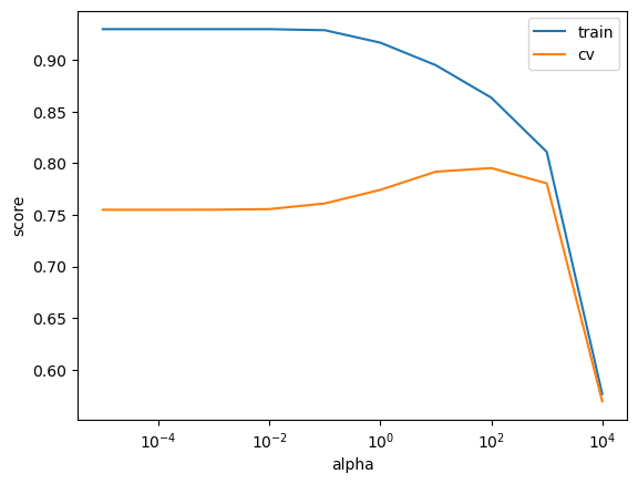
best_alpha = search.best_params_
best_alpha
{'ridge__alpha': 100.0}
search.best_score_
0.7951559890417758
It seems alpha=100 is the best choice here.
General intuition: larger
alphaleads to smaller coefficients.Smaller coefficients mean the predictions are less sensitive to changes in the data. Hence less chance of overfitting.
pipe_bigalpha = make_pipeline(preprocessor, Ridge(alpha=1000))
pipe_bigalpha.fit(X_train, y_train)
bigalpha_coeffs = pipe_bigalpha.named_steps["ridge"].coef_
pd.DataFrame(
    data=bigalpha_coeffs, index=new_columns, columns=["Coefficients"]
).sort_values(by="Coefficients", ascending=False)
| Coefficients | |
|---|---|
| OverallQual | 9691.378159 |
| GrLivArea | 7816.490033 |
| 1stFlrSF | 5931.401623 |
| TotRmsAbvGrd | 5209.377032 |
| GarageCars | 5057.215412 |
| ... | ... |
| SaleType_WD | -1214.532034 |
| GarageFinish_Unf | -1281.596864 |
| Foundation_CBlock | -1766.048889 |
| RoofStyle_Gable | -1985.253914 |
| KitchenAbvGr | -2623.509001 |
262 rows × 1 columns
Smaller
alphaleads to bigger coefficients.
pipe_smallalpha = make_pipeline(preprocessor, Ridge(alpha=0.01))
pipe_smallalpha.fit(X_train, y_train)
smallalpha_coeffs = pipe_smallalpha.named_steps["ridge"].coef_
pd.DataFrame(
    data=smallalpha_coeffs, index=new_columns, columns=["Coefficients"]
).sort_values(by="Coefficients", ascending=False)
| Coefficients | |
|---|---|
| RoofMatl_WdShngl | 128384.117412 |
| RoofMatl_Membran | 127326.497787 |
| RoofMatl_Metal | 106023.481515 |
| Condition2_PosA | 83437.787574 |
| RoofMatl_CompShg | 70568.838951 |
| ... | ... |
| Exterior1st_ImStucc | -34441.626206 |
| Heating_OthW | -34806.290424 |
| Condition2_RRAe | -63362.335309 |
| Condition2_PosN | -194985.470060 |
| RoofMatl_ClyTile | -582469.424221 |
262 rows × 1 columns
With the best alpha found by the grid search, the coefficients are somewhere in between.
pipe_bestalpha = make_pipeline(
    preprocessor, Ridge(alpha=search.best_params_["ridge__alpha"])
)
pipe_bestalpha.fit(X_train, y_train)
bestalpha_coeffs = pipe_bestalpha.named_steps["ridge"].coef_
pd.DataFrame(
    data=bestalpha_coeffs, index=new_columns, columns=["Coefficients"]
).sort_values(by="Coefficients", ascending=False)
| Coefficients | |
|---|---|
| OverallQual | 14485.526602 |
| GrLivArea | 11693.792577 |
| Neighborhood_NridgHt | 9661.926657 |
| Neighborhood_NoRidge | 9492.921850 |
| BsmtQual | 8076.988901 |
| ... | ... |
| RoofMatl_ClyTile | -3991.413796 |
| LandContour_Bnk | -5002.470666 |
| Neighborhood_Gilbert | -5212.984664 |
| Neighborhood_CollgCr | -5461.450739 |
| Neighborhood_Edwards | -5789.889086 |
262 rows × 1 columns
To summarize:
Higher values of
alphameans a more restricted model.The values of coefficients are likely to be smaller for higher values of
alphacompared to lower values of alpha.
RidgeCV#
Because it’s so common to want to tune alpha with Ridge, sklearn provides a class called RidgeCV, which automatically tunes alpha based on cross-validation.
alphas = 10.0 ** np.arange(-6, 6, 1)
ridgecv_pipe = make_pipeline(preprocessor, RidgeCV(alphas=alphas, cv=10))
ridgecv_pipe.fit(X_train, y_train);
best_alpha = ridgecv_pipe.named_steps["ridgecv"].alpha_

best_alpha
100.0
Let’s examine the tuned model.
ridge_tuned = make_pipeline(preprocessor, Ridge(alpha=best_alpha))
ridge_tuned.fit(X_train, y_train)
ridge_preds = ridge_tuned.predict(X_test)
ridge_preds[:10]
array([228603.06797961, 104643.99931883, 155624.61029914, 246332.07245741,
       127614.33726089, 243243.60429913, 304784.87844893, 145425.67512181,
       157008.6526853 , 128528.91515735])
df = pd.DataFrame(
    data={"coefficients": ridge_tuned.named_steps["ridge"].coef_}, index=new_columns
)
df.sort_values("coefficients", ascending=False)
| coefficients | |
|---|---|
| OverallQual | 14485.526602 |
| GrLivArea | 11693.792577 |
| Neighborhood_NridgHt | 9661.926657 |
| Neighborhood_NoRidge | 9492.921850 |
| BsmtQual | 8076.988901 |
| ... | ... |
| RoofMatl_ClyTile | -3991.413796 |
| LandContour_Bnk | -5002.470666 |
| Neighborhood_Gilbert | -5212.984664 |
| Neighborhood_CollgCr | -5461.450739 |
| Neighborhood_Edwards | -5789.889086 |
262 rows × 1 columns
So according to this model:
As
OverallQualfeature gets bigger the housing price will get bigger.Neighborhood_Edwardsis associated with reducing the housing price.We’ll talk more about interpretation of different kinds of features next week.
ridge_preds.max(), ridge_preds.min()
(390725.7472092076, 30815.281220255274)
❓❓ Questions for you#
iClicker Exercise 10.1#
iClicker cloud join link: https://join.iclicker.com/SNBF
Select all of the following statements which are TRUE.
(A) Price per square foot would be a good feature to add in our
X.(B) The
alphahyperparameter ofRidgehas similar interpretation ofChyperparameter ofLogisticRegression; higheralphameans more complex model.(C) In
Ridge, smaller alpha means bigger coefficients whereas bigger alpha means smaller coefficients.
Can we use the metrics we looked at in the previous lecture for this problem? Why or why not?
Regression scoring functions#
We aren’t doing classification anymore, so we can’t just check for equality:
ridge_tuned.predict(X_train) == y_train
302     False
767     False
429     False
1139    False
558     False
        ...
1041    False
1122    False
1346    False
1406    False
1389    False
Name: SalePrice, Length: 1314, dtype: bool
y_train.values
array([205000, 160000, 175000, ..., 262500, 133000, 131000])
ridge_tuned.predict(X_train)
array([212870.41150573, 178494.22221894, 189981.34426571, ...,
       245329.56804591, 129904.71327467, 135422.67672595])
We need a score that reflects how right/wrong each prediction is.
There are a number of popular scoring functions for regression. We are going to look at some common metrics:
mean squared error (MSE)
\(R^2\)
root mean squared error (RMSE)
MAPE
See sklearn documentation for more details.
Mean squared error (MSE)#
A common metric is mean squared error:
preds = ridge_tuned.predict(X_train)
np.mean((y_train - preds) ** 2)
872961060.7986538
Perfect predictions would have MSE=0.
np.mean((y_train - y_train) ** 2)
0.0
This is also implemented in sklearn:
from sklearn.metrics import mean_squared_error

mean_squared_error(y_train, preds)
872961060.7986538
MSE looks huge and unreasonable. There is an error of ~$1 Billion!
Is this score good or bad?
Unlike classification, with regression our target has units.
The target is in dollars, the mean squared error is in \(dollars^2\)
The score also depends on the scale of the targets.
If we were working in cents instead of dollars, our MSE would be \(10,000 \times (100^2\)) higher!
np.mean((y_train * 100 - preds * 100) ** 2)
8729610607986.539
Root mean squared error or RMSE#
The MSE above is in \(dollars^2\).
A more relatable metric would be the root mean squared error, or RMSE
np.sqrt(mean_squared_error(y_train, ridge_tuned.predict(X_train)))
29545.914451894256
Error of $30,000 makes more sense.
Let’s dig deeper.
plt.scatter(y_train, ridge_tuned.predict(X_train), alpha=0.3)
grid = np.linspace(y_train.min(), y_train.max(), 1000)
plt.plot(grid, grid, "--k")
plt.xlabel("true price")
plt.ylabel("predicted price");
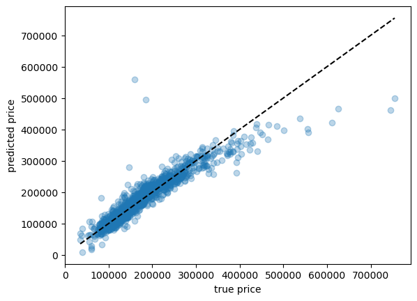
Here we can see a few cases where our prediction is way off.
Is there something weird about those houses, perhaps? Outliers?
Under the line means we’re under-predicting, over the line means we’re over-predicting.
\(R^2\) (not in detail)#
A common score is the \(R^2\)
This is the score that
sklearnuses by default when you call score()You can read about it if interested.
\(R^2\) measures the proportion of variability in \(y\) that can be explained using \(X\).
Independent of the scale of \(y\). So the max is 1.
The denominator measures the total variance in \(y\).
The amount of variability that is left unexplained after performing regression.
Key points:
The maximum is 1 for perfect predictions
Negative values are very bad: “worse than DummyRegressor” (very bad)
(Optional) Warning: MSE is “reversible” but \(R^2\) is not:
mean_squared_error(y_train, preds)
872961060.7986538
mean_squared_error(preds, y_train)
872961060.7986538
r2_score(y_train, preds)
0.8601643854446083
r2_score(preds, y_train)
0.8280229354283184
When you call
fitit minimizes MSE / maximizes \(R^2\) (or something like that) by default.Just like in classification, this isn’t always what you want!!
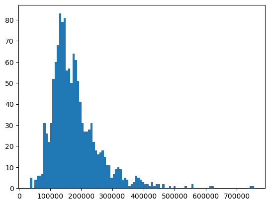
MAPE#
We got an RMSE of ~$30,000 before.
Question: Is an error of $30,000 acceptable?
np.sqrt(mean_squared_error(y_train, ridge_tuned.predict(X_train)))
29545.914451894256
For a house worth $600k, it seems reasonable! That’s 5% error.
For a house worth $60k, that is terrible. It’s 50% error.
We have both of these cases in our dataset.
plt.hist(y_train, bins=100);
How about looking at percent error?
pred_train = ridge_tuned.predict(X_train)
percent_errors = (pred_train - y_train) / y_train * 100.0
percent_errors
302      3.839225
767     11.558889
429      8.560768
1139   -16.405650
558     17.194710
          ...
1041    -0.496213
1122   -28.624615
1346    -6.541117
1406    -2.327283
1389     3.376089
Name: SalePrice, Length: 1314, dtype: float64
These are both positive (predict too high) and negative (predict too low).
We can look at the absolute percent error:
np.abs(percent_errors)
302      3.839225
767     11.558889
429      8.560768
1139    16.405650
558     17.194710
          ...
1041     0.496213
1122    28.624615
1346     6.541117
1406     2.327283
1389     3.376089
Name: SalePrice, Length: 1314, dtype: float64
And, like MSE, we can take the average over examples. This is called mean absolute percent error (MAPE).
def my_mape(true, pred):
    return np.mean(np.abs((pred - true) / true))
my_mape(y_train, pred_train)
0.10092665203438773
Let’s use sklearn to calculate MAPE.
from sklearn.metrics import mean_absolute_percentage_error
mean_absolute_percentage_error(y_train, pred_train)
0.10092665203438773
Ok, this is quite interpretable.
On average, we have around 10% error.
Transforming the targets#
When you have prices or count data, the target values are skewed.
Let’s look at our target column.
plt.hist(y_train, bins=100);
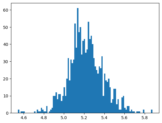
A common trick in such cases is applying a log transform on the target column to make it more normal and less skewed.
That is, transform \(y\rightarrow \log(y)\).
Linear regression will usually work better on something that looks more normal.
plt.hist(np.log10(y_train), bins=100);
We can incorporate this in our pipeline using sklearn.
from sklearn.compose import TransformedTargetRegressor
ttr = TransformedTargetRegressor(
    Ridge(alpha=best_alpha), func=np.log1p, inverse_func=np.expm1
) # transformer for log transforming the target
ttr_pipe = make_pipeline(preprocessor, ttr)
ttr_pipe
Pipeline(steps=[('columntransformer',
                 ColumnTransformer(transformers=[('drop', 'drop', ['Id']),
                                                 ('pipeline-1',
                                                  Pipeline(steps=[('simpleimputer',
                                                                   SimpleImputer(strategy='median')),
                                                                  ('standardscaler',
                                                                   StandardScaler())]),
                                                  ['BedroomAbvGr',
                                                   'KitchenAbvGr',
                                                   'LotFrontage', 'LotArea',
                                                   'OverallQual', 'OverallCond',
                                                   'YearBuilt', 'YearRemodAdd',
                                                   'MasVnrArea', 'BsmtFinSF1',
                                                   'Bs...
                                                   'HouseStyle', 'Heating',
                                                   'LandSlope', 'Utilities',
                                                   'Electrical', 'RoofStyle',
                                                   'MiscFeature', 'MoSold',
                                                   'Exterior1st', 'Alley',
                                                   'SaleCondition',
                                                   'Neighborhood', 'Foundation',
                                                   'MSZoning', 'LotConfig',
                                                   'MasVnrType',
                                                   'MSSubClass'])])),
                ('transformedtargetregressor',
                 TransformedTargetRegressor(func=<ufunc 'log1p'>,
                                            inverse_func=<ufunc 'expm1'>,
                                            regressor=Ridge(alpha=100.0)))])
In a Jupyter environment, please rerun this cell to show the HTML representation or trust the notebook. On GitHub, the HTML representation is unable to render, please try loading this page with nbviewer.org.
Pipeline(steps=[('columntransformer',
                 ColumnTransformer(transformers=[('drop', 'drop', ['Id']),
                                                 ('pipeline-1',
                                                  Pipeline(steps=[('simpleimputer',
                                                                   SimpleImputer(strategy='median')),
                                                                  ('standardscaler',
                                                                   StandardScaler())]),
                                                  ['BedroomAbvGr',
                                                   'KitchenAbvGr',
                                                   'LotFrontage', 'LotArea',
                                                   'OverallQual', 'OverallCond',
                                                   'YearBuilt', 'YearRemodAdd',
                                                   'MasVnrArea', 'BsmtFinSF1',
                                                   'Bs...
                                                   'HouseStyle', 'Heating',
                                                   'LandSlope', 'Utilities',
                                                   'Electrical', 'RoofStyle',
                                                   'MiscFeature', 'MoSold',
                                                   'Exterior1st', 'Alley',
                                                   'SaleCondition',
                                                   'Neighborhood', 'Foundation',
                                                   'MSZoning', 'LotConfig',
                                                   'MasVnrType',
                                                   'MSSubClass'])])),
                ('transformedtargetregressor',
                 TransformedTargetRegressor(func=<ufunc 'log1p'>,
                                            inverse_func=<ufunc 'expm1'>,
regressor=Ridge(alpha=100.0)))])ColumnTransformer(transformers=[('drop', 'drop', ['Id']),
('pipeline-1',
Pipeline(steps=[('simpleimputer',
SimpleImputer(strategy='median')),
('standardscaler',
StandardScaler())]),
['BedroomAbvGr', 'KitchenAbvGr', 'LotFrontage',
'LotArea', 'OverallQual', 'OverallCond',
'YearBuilt', 'YearRemodAdd', 'MasVnrArea',
'BsmtFinSF1', 'BsmtFinSF2', 'BsmtUnfSF',
'TotalBsmtSF', '...
['GarageFinish', 'LandContour', 'LotShape',
'Condition1', 'Condition2', 'SaleType',
'Exterior2nd', 'CentralAir', 'PavedDrive',
'RoofMatl', 'Street', 'BldgType',
'GarageType', 'HouseStyle', 'Heating',
'LandSlope', 'Utilities', 'Electrical',
'RoofStyle', 'MiscFeature', 'MoSold',
'Exterior1st', 'Alley', 'SaleCondition',
'Neighborhood', 'Foundation', 'MSZoning',
'LotConfig', 'MasVnrType', 'MSSubClass'])])['Id']
drop
['BedroomAbvGr', 'KitchenAbvGr', 'LotFrontage', 'LotArea', 'OverallQual', 'OverallCond', 'YearBuilt', 'YearRemodAdd', 'MasVnrArea', 'BsmtFinSF1', 'BsmtFinSF2', 'BsmtUnfSF', 'TotalBsmtSF', '1stFlrSF', '2ndFlrSF', 'LowQualFinSF', 'GrLivArea', 'BsmtFullBath', 'BsmtHalfBath', 'FullBath', 'HalfBath', 'TotRmsAbvGrd', 'Fireplaces', 'GarageYrBlt', 'GarageCars', 'GarageArea', 'WoodDeckSF', 'OpenPorchSF', 'EnclosedPorch', '3SsnPorch', 'ScreenPorch', 'PoolArea', 'MiscVal', 'YrSold']
SimpleImputer(strategy='median')
StandardScaler()
['ExterQual', 'ExterCond', 'BsmtQual', 'BsmtCond', 'HeatingQC', 'KitchenQual', 'FireplaceQu', 'GarageQual', 'GarageCond', 'PoolQC']
SimpleImputer(strategy='most_frequent')
OrdinalEncoder(categories=[['Po', 'Fa', 'TA', 'Gd', 'Ex'],
                           ['Po', 'Fa', 'TA', 'Gd', 'Ex'],
                           ['Po', 'Fa', 'TA', 'Gd', 'Ex'],
                           ['Po', 'Fa', 'TA', 'Gd', 'Ex'],
                           ['Po', 'Fa', 'TA', 'Gd', 'Ex'],
                           ['Po', 'Fa', 'TA', 'Gd', 'Ex'],
                           ['Po', 'Fa', 'TA', 'Gd', 'Ex'],
                           ['Po', 'Fa', 'TA', 'Gd', 'Ex'],
                           ['Po', 'Fa', 'TA', 'Gd', 'Ex'],
['Po', 'Fa', 'TA', 'Gd', 'Ex']])['BsmtExposure', 'BsmtFinType1', 'BsmtFinType2', 'Functional', 'Fence']
SimpleImputer(strategy='most_frequent')
OrdinalEncoder(categories=[['NA', 'No', 'Mn', 'Av', 'Gd'],
                           ['NA', 'Unf', 'LwQ', 'Rec', 'BLQ', 'ALQ', 'GLQ'],
                           ['NA', 'Unf', 'LwQ', 'Rec', 'BLQ', 'ALQ', 'GLQ'],
                           ['Sal', 'Sev', 'Maj2', 'Maj1', 'Mod', 'Min2', 'Min1',
                            'Typ'],
['NA', 'MnWw', 'GdWo', 'MnPrv', 'GdPrv']])['GarageFinish', 'LandContour', 'LotShape', 'Condition1', 'Condition2', 'SaleType', 'Exterior2nd', 'CentralAir', 'PavedDrive', 'RoofMatl', 'Street', 'BldgType', 'GarageType', 'HouseStyle', 'Heating', 'LandSlope', 'Utilities', 'Electrical', 'RoofStyle', 'MiscFeature', 'MoSold', 'Exterior1st', 'Alley', 'SaleCondition', 'Neighborhood', 'Foundation', 'MSZoning', 'LotConfig', 'MasVnrType', 'MSSubClass']
SimpleImputer(fill_value='missing', strategy='constant')
OneHotEncoder(handle_unknown='ignore', sparse_output=False)
TransformedTargetRegressor(func=<ufunc 'log1p'>, inverse_func=<ufunc 'expm1'>,
regressor=Ridge(alpha=100.0))Ridge(alpha=100.0)
Ridge(alpha=100.0)
Why can’t we incorporate preprocessing targets in our column transformer?
ttr_pipe.fit(X_train, y_train); # y_train automatically transformed
ttr_pipe.predict(X_train) # predictions automatically un-transformed
array([221329.43833466, 170670.12761659, 182639.31984311, ...,
       248609.60023631, 132158.15026771, 133270.71866979])
mean_absolute_percentage_error(y_test, ttr_pipe.predict(X_test))
0.07808506982896271
We reduced MAPE from ~10% to ~8% with this trick!
Does
.fit()know we care about MAPE?No, it doesn’t. Why are we minimizing MSE (or something similar) if we care about MAPE??
When minimizing MSE, the expensive houses will dominate because they have the biggest error.
Different scoring functions with cross_validate#
Let’s try using MSE instead of the default \(R^2\) score.
pd.DataFrame(
    cross_validate(
        ridge_tuned,
        X_train,
        y_train,
        return_train_score=True,
        scoring="neg_mean_squared_error",
    )
)
| fit_time | score_time | test_score | train_score | |
|---|---|---|---|---|
| 0 | 0.025777 | 0.006925 | -7.055915e+08 | -9.379875e+08 |
| 1 | 0.024397 | 0.006842 | -1.239944e+09 | -8.264283e+08 |
| 2 | 0.024002 | 0.006774 | -1.125440e+09 | -8.758062e+08 |
| 3 | 0.024273 | 0.006692 | -9.801219e+08 | -8.849438e+08 |
| 4 | 0.024040 | 0.006704 | -2.267612e+09 | -7.395282e+08 |
# make a scorer function that we can pass into cross-validation
mape_scorer = make_scorer(my_mape, greater_is_better=False)

pd.DataFrame(
    cross_validate(
        ridge_tuned, X_train, y_train, return_train_score=True, scoring=mape_scorer
    )
)
| fit_time | score_time | test_score | train_score | |
|---|---|---|---|---|
| 0 | 0.024928 | 0.006840 | -0.096960 | -0.104070 |
| 1 | 0.024294 | 0.007623 | -0.107985 | -0.099685 |
| 2 | 0.024001 | 0.006786 | -0.118347 | -0.101796 |
| 3 | 0.024005 | 0.006607 | -0.107947 | -0.102435 |
| 4 | 0.025644 | 0.006638 | -0.121985 | -0.098307 |
If you are finding greater_is_better=False argument confusing, here is the documentation:
greater_is_better(bool), default=True Whether score_func is a score function (default), meaning high is good, or a loss function, meaning low is good. In the latter case, the scorer object will sign-flip the outcome of the score_func.
Since our custom scorer mape gives an error and not a score, I’m passing False to it and it’ll sign flip so that we can interpret bigger numbers as better performance.
# ?make_scorer
scoring = {
    "r2": "r2",
    "mape_scorer": mape_scorer, # just for demonstration for a custom scorer
    "sklearn MAPE": "neg_mean_absolute_percentage_error",
    "neg_root_mean_square_error": "neg_root_mean_squared_error",
    "neg_mean_squared_error": "neg_mean_squared_error",
}

pd.DataFrame(
    cross_validate(
        ridge_tuned, X_train, y_train, return_train_score=True, scoring=scoring
    )
).T
| 0 | 1 | 2 | 3 | 4 | |
|---|---|---|---|---|---|
| fit_time | 2.595615e-02 | 2.484584e-02 | 2.470708e-02 | 2.400208e-02 | 2.449203e-02 |
| score_time | 8.028984e-03 | 8.161068e-03 | 8.410931e-03 | 7.450104e-03 | 7.692099e-03 |
| test_r2 | 8.669805e-01 | 8.200326e-01 | 8.262156e-01 | 8.514598e-01 | 6.110915e-01 |
| train_r2 | 8.551862e-01 | 8.636849e-01 | 8.580539e-01 | 8.561645e-01 | 8.834356e-01 |
| test_mape_scorer | -9.696034e-02 | -1.079852e-01 | -1.183471e-01 | -1.079471e-01 | -1.219845e-01 |
| train_mape_scorer | -1.040698e-01 | -9.968514e-02 | -1.017959e-01 | -1.024351e-01 | -9.830712e-02 |
| test_sklearn MAPE | -9.696034e-02 | -1.079852e-01 | -1.183471e-01 | -1.079471e-01 | -1.219845e-01 |
| train_sklearn MAPE | -1.040698e-01 | -9.968514e-02 | -1.017959e-01 | -1.024351e-01 | -9.830712e-02 |
| test_neg_root_mean_square_error | -2.656297e+04 | -3.521284e+04 | -3.354759e+04 | -3.130690e+04 | -4.761945e+04 |
| train_neg_root_mean_square_error | -3.062658e+04 | -2.874767e+04 | -2.959402e+04 | -2.974801e+04 | -2.719427e+04 |
| test_neg_mean_squared_error | -7.055915e+08 | -1.239944e+09 | -1.125440e+09 | -9.801219e+08 | -2.267612e+09 |
| train_neg_mean_squared_error | -9.379875e+08 | -8.264283e+08 | -8.758062e+08 | -8.849438e+08 | -7.395282e+08 |
Are we getting the same alpha with mape?
param_grid = {"ridge__alpha": 10.0 ** np.arange(-6, 6, 1)}

pipe_ridge = make_pipeline(preprocessor, Ridge())

search = GridSearchCV(
    pipe_ridge, param_grid, return_train_score=True, n_jobs=-1, scoring=mape_scorer
)
search.fit(X_train, y_train);
print("Best hyperparameter values: ", search.best_params_)
print("Best score: %0.3f" % (search.best_score_))
pd.DataFrame(search.cv_results_)[
    [
        "mean_train_score",
        "mean_test_score",
        "param_ridge__alpha",
        "mean_fit_time",
        "rank_test_score",
    ]
].set_index("rank_test_score").sort_index().T
Best hyperparameter values:  {'ridge__alpha': 100.0}
Best score: -0.111
| rank_test_score | 1 | 2 | 3 | 4 | 5 | 6 | 7 | 8 | 9 | 10 | 11 | 12 |
|---|---|---|---|---|---|---|---|---|---|---|---|---|
| mean_train_score | -0.101259 | -0.111543 | -0.096462 | -0.090785 | -0.085698 | -0.085508 | -0.085546 | -0.08555 | -0.085551 | -0.085551 | -0.203421 | -0.33213 |
| mean_test_score | -0.110645 | -0.115401 | -0.116497 | -0.122331 | -0.125644 | -0.127242 | -0.127418 | -0.127439 | -0.127441 | -0.127441 | -0.204692 | -0.33271 |
| param_ridge__alpha | 100.0 | 1000.0 | 10.0 | 1.0 | 0.1 | 0.01 | 0.001 | 0.0001 | 0.00001 | 0.000001 | 10000.0 | 100000.0 |
| mean_fit_time | 0.035483 | 0.038616 | 0.040649 | 0.045599 | 0.040408 | 0.041231 | 0.039581 | 0.04547 | 0.038408 | 0.032273 | 0.041343 | 0.037057 |
Using multiple metrics in GridSearchCV or RandomizedSearchCV#
We could use multiple metrics with
GridSearchCVorRandomizedSearchCV.But if you do so, you need to set
refitto the metric (string) for which thebest_params_will be found and used to build thebest_estimator_on the whole dataset.
search_multi = GridSearchCV(
    pipe_ridge,
    param_grid,
    return_train_score=True,
    n_jobs=-1,
    scoring=scoring,
    refit="sklearn MAPE",
)
search_multi.fit(X_train, y_train);
print("Best hyperparameter values: ", search_multi.best_params_)
print("Best score: %0.3f" % (search_multi.best_score_))
pd.DataFrame(search_multi.cv_results_).set_index("rank_test_mape_scorer").sort_index()
Best hyperparameter values:  {'ridge__alpha': 100.0}
Best score: -0.111
| mean_fit_time | std_fit_time | mean_score_time | std_score_time | param_ridge__alpha | params | split0_test_r2 | split1_test_r2 | split2_test_r2 | split3_test_r2 | ... | mean_test_neg_mean_squared_error | std_test_neg_mean_squared_error | rank_test_neg_mean_squared_error | split0_train_neg_mean_squared_error | split1_train_neg_mean_squared_error | split2_train_neg_mean_squared_error | split3_train_neg_mean_squared_error | split4_train_neg_mean_squared_error | mean_train_neg_mean_squared_error | std_train_neg_mean_squared_error | |
|---|---|---|---|---|---|---|---|---|---|---|---|---|---|---|---|---|---|---|---|---|---|
| rank_test_mape_scorer | |||||||||||||||||||||
| 1 | 0.041573 | 0.004271 | 0.013070 | 0.002356 | 100.0 | {'ridge__alpha': 100.0} | 0.866980 | 0.820033 | 0.826216 | 0.851460 | ... | -1.263742e+09 | 5.328077e+08 | 1 | -9.379875e+08 | -8.264283e+08 | -8.758062e+08 | -8.849438e+08 | -7.395282e+08 | -8.529388e+08 | 6.685103e+07 |
| 2 | 0.039553 | 0.003296 | 0.011070 | 0.003513 | 1000.0 | {'ridge__alpha': 1000.0} | 0.827261 | 0.786555 | 0.802902 | 0.812272 | ... | -1.362185e+09 | 3.262269e+08 | 3 | -1.282021e+09 | -1.156311e+09 | -1.207814e+09 | -1.225301e+09 | -1.029950e+09 | -1.180279e+09 | 8.521743e+07 |
| 3 | 0.037233 | 0.003226 | 0.014097 | 0.002145 | 10.0 | {'ridge__alpha': 10.0} | 0.859318 | 0.820564 | 0.832866 | 0.846650 | ... | -1.283119e+09 | 5.511620e+08 | 2 | -7.034979e+08 | -6.276943e+08 | -6.910456e+08 | -6.701186e+08 | -5.915714e+08 | -6.567856e+08 | 4.155178e+07 |
| 4 | 0.042143 | 0.003760 | 0.011983 | 0.003802 | 1.0 | {'ridge__alpha': 1.0} | 0.835749 | 0.810073 | 0.831611 | 0.843992 | ... | -1.386071e+09 | 6.378971e+08 | 4 | -5.394113e+08 | -4.898703e+08 | -5.405227e+08 | -5.290961e+08 | -5.046193e+08 | -5.207039e+08 | 2.011269e+07 |
| 5 | 0.041837 | 0.002342 | 0.012658 | 0.003056 | 0.1 | {'ridge__alpha': 0.1} | 0.821807 | 0.792828 | 0.805198 | 0.863941 | ... | -1.465279e+09 | 6.931439e+08 | 5 | -4.579559e+08 | -4.009514e+08 | -4.345386e+08 | -4.515351e+08 | -4.846260e+08 | -4.459214e+08 | 2.766317e+07 |
| 6 | 0.036263 | 0.003491 | 0.017713 | 0.002790 | 0.01 | {'ridge__alpha': 0.01} | 0.824884 | 0.782183 | 0.787933 | 0.868003 | ... | -1.501304e+09 | 7.090376e+08 | 6 | -4.522563e+08 | -3.926733e+08 | -4.251158e+08 | -4.446284e+08 | -4.837022e+08 | -4.396752e+08 | 3.014081e+07 |
| 7 | 0.038944 | 0.004208 | 0.012339 | 0.002726 | 0.001 | {'ridge__alpha': 0.001} | 0.826553 | 0.780497 | 0.785399 | 0.868281 | ... | -1.505592e+09 | 7.117899e+08 | 7 | -4.521578e+08 | -3.925288e+08 | -4.249618e+08 | -4.445124e+08 | -4.836880e+08 | -4.395697e+08 | 3.018459e+07 |
| 8 | 0.036164 | 0.004368 | 0.013690 | 0.001376 | 0.0001 | {'ridge__alpha': 0.0001} | 0.826739 | 0.780316 | 0.785134 | 0.868305 | ... | -1.506035e+09 | 7.120769e+08 | 8 | -4.521567e+08 | -3.925272e+08 | -4.249601e+08 | -4.445111e+08 | -4.836878e+08 | -4.395686e+08 | 3.018507e+07 |
| 9 | 0.038126 | 0.004525 | 0.012731 | 0.003667 | 0.00001 | {'ridge__alpha': 1e-05} | 0.826758 | 0.780298 | 0.785108 | 0.868308 | ... | -1.506079e+09 | 7.121056e+08 | 9 | -4.521567e+08 | -3.925272e+08 | -4.249601e+08 | -4.445111e+08 | -4.836878e+08 | -4.395686e+08 | 3.018507e+07 |
| 10 | 0.031822 | 0.003929 | 0.012328 | 0.003792 | 0.000001 | {'ridge__alpha': 1e-06} | 0.826760 | 0.780296 | 0.785105 | 0.868308 | ... | -1.506084e+09 | 7.121084e+08 | 10 | -4.521567e+08 | -3.925272e+08 | -4.249601e+08 | -4.445111e+08 | -4.836878e+08 | -4.395686e+08 | 3.018507e+07 |
| 11 | 0.040749 | 0.002128 | 0.011912 | 0.003928 | 10000.0 | {'ridge__alpha': 10000.0} | 0.593370 | 0.551975 | 0.568663 | 0.557739 | ... | -2.686348e+09 | 3.316395e+08 | 11 | -2.762093e+09 | -2.571901e+09 | -2.662541e+09 | -2.624450e+09 | -2.595569e+09 | -2.643311e+09 | 6.665351e+07 |
| 12 | 0.037351 | 0.002842 | 0.009640 | 0.003145 | 100000.0 | {'ridge__alpha': 100000.0} | 0.135384 | 0.113837 | 0.118874 | 0.123367 | ... | -5.442377e+09 | 5.531116e+08 | 12 | -5.629792e+09 | -5.271738e+09 | -5.379416e+09 | -5.342605e+09 | -5.498133e+09 | -5.424337e+09 | 1.262079e+08 |
12 rows × 80 columns
What’s the test score?
search_multi.score(X_test, y_test)
-0.09503409246217502
my_mape(y_test, ridge_tuned.predict(X_test))
0.09503409246217502
Using regression metrics with scikit-learn#
In
sklearn, you will notice that it has negative version of the metrics above (e.g.,neg_mean_squared_error,neg_root_mean_squared_error).The reason for this is that scores return a value to maximize, the higher the better.
❓❓ Questions for you#
iClicker Exercise 10.2#
iClicker cloud join link: https://join.iclicker.com/SNBF
Select all of the following statements which are TRUE.
(A) We can use still use precision and recall for regression problems but now we have other metrics we can use as well.
(B) In
sklearnfor regression problems, usingr2_score()and.score()(with default values) will produce the same results.(C) RMSE is always going to be non-negative.
(D) MSE does not directly provide the information about whether the model is underpredicting or overpredicting.
(E) We can pass multiple scoring metrics to
GridSearchCVorRandomizedSearchCVfor regression as well as classification problems.
What did we learn today?#
House prices dataset target is price, which is numeric -> regression rather than classification
There are corresponding versions of all the tools we used:
DummyClassifier->DummyRegressorLogisticRegression->Ridge
Ridgehyperparameteralphais likeLogisticRegressionhyperparameterC, but opposite meaningWe’ll avoid
LinearRegressionin this course.
Scoring metrics
\(R^2\) is the default .score(), it is unitless, 0 is bad, 1 is best
MSE (mean squared error) is in units of target squared, hard to interpret; 0 is best
RMSE (root mean squared error) is in the same units as the target; 0 is best
MAPE (mean absolute percent error) is unitless; 0 is best, 1 is bad