Lecture 4: \(k\)-Nearest Neighbours and SVM RBFs

UBC 2023-24

Instructor: Varada Kolhatkar and Andrew Roth

If two things are similar, the thought of one will tend to trigger the thought of the other
– Aristotle

Lecture plan

• Announcements

• Recap: Lecture 3 iClicker questions (~15 mins)

• iClicker questions (~10 mins)

• Class demo (~20 mins)

• Break (~5 mins)

• Worksheet (~25 mins)

Imports, announcements, and LOs

Imports

import sys

import IPython
import matplotlib.pyplot as plt
import numpy as np
import pandas as pd
from IPython.display import HTML

sys.path.append("code/.")

import ipywidgets as widgets
import mglearn
from IPython.display import display
from ipywidgets import interact, interactive
from plotting_functions import *
from sklearn.dummy import DummyClassifier
from sklearn.model_selection import cross_validate, train_test_split
from utils import *

%matplotlib inline

pd.set_option("display.max_colwidth", 200)
import warnings

warnings.filterwarnings("ignore")

Announcements

• hw2 was due yesterday.

• hw3 is released. (Due Monday, October 2nd at 11:59pm.)

  • We are allowing group submissions for this homework.

• The lecture notes within these notebooks align with the content presented in the videos. Even though we do not cover all the content from these notebooks during lectures, it’s your responsibility to go through them on your own.

• By this point, you should know your course enrollment status. Registration for tutorials is not mandatory; they are optional and will follow an office-hour format. You are free to attend any tutorial session of your choice.

Learning outcomes

From this lecture, you will be able to

• explain the notion of similarity-based algorithms;

• broadly describe how \(k\)-NNs use distances;

• discuss the effect of using a small/large value of the hyperparameter \(k\) when using the \(k\)-NN algorithm;

• describe the problem of curse of dimensionality;

• explain the general idea of SVMs with RBF kernel;

• broadly describe the relation of gamma and C hyperparameters of SVMs with the fundamental tradeoff.

Quick recap

• Why do we split the data?

• What are the 4 types of data we discussed last class?

• What are the benefits of cross-validation?

• What is overfitting?

• What’s the fundamental trade-off in supervised machine learning?

• What is the golden rule of machine learning?

Important

If you want to run this notebook you will have to install ipywidgets. Follow the installation instructions here.

Motivation and distances [video]

Analogy-based models

• Suppose you are given the following training examples with corresponding labels and are asked to label a given test example.

source

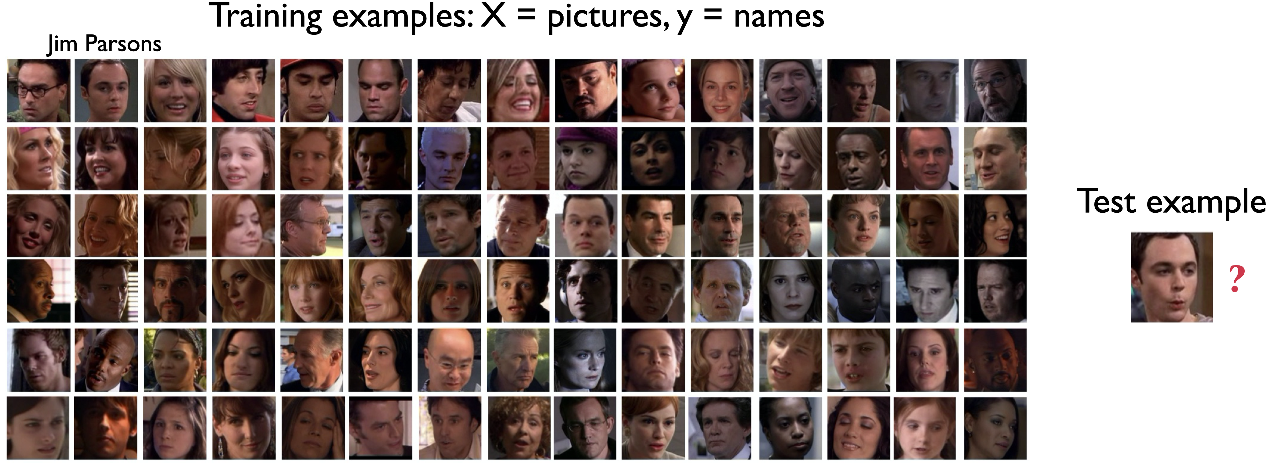
• An intuitive way to classify the test example is by finding the most “similar” example(s) from the training set and using that label for the test example.

Analogy-based algorithms in practice

• Herta’s High-tech Facial Recognition

  • Feature vectors for human faces

  • \(k\)-NN to identify which face is on their watch list

• Recommendation systems

General idea of \(k\)-nearest neighbours algorithm

• Consider the following toy dataset with two classes.

  • blue circles \(\rightarrow\) class 0

  • red triangles \(\rightarrow\) class 1

  • green stars \(\rightarrow\) test examples

X, y = mglearn.datasets.make_forge()
X_test = np.array([[8.2, 3.66214339], [9.9, 3.2], [11.2, 0.5]])

plot_train_test_points(X, y, X_test)

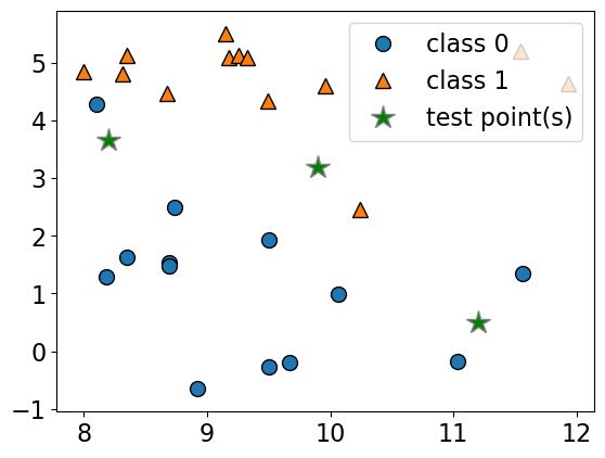
• Given a new data point, predict the class of the data point by finding the “closest” data point in the training set, i.e., by finding its “nearest neighbour” or majority vote of nearest neighbours.

def f(n_neighbors):
    return plot_knn_clf(X, y, X_test, n_neighbors=n_neighbors)

interactive(
    f,
    n_neighbors=widgets.IntSlider(min=1, max=10, step=2, value=1),
)

Geometric view of tabular data and dimensions

• To understand analogy-based algorithms it’s useful to think of data as points in a high dimensional space.

• Our X represents the problem in terms of relevant features (\(d\)) with one dimension for each feature (column).

• Examples are points in a \(d\)-dimensional space.

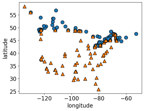
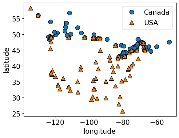
How many dimensions (features) are there in the cities data?

cities_df = pd.read_csv("data/canada_usa_cities.csv")
X_cities = cities_df[["longitude", "latitude"]]
y_cities = cities_df["country"]

mglearn.discrete_scatter(X_cities.iloc[:, 0], X_cities.iloc[:, 1], y_cities)
plt.xlabel("longitude")
plt.ylabel("latitude");

• Recall the Spotify Song Attributes dataset from homework 1.

• How many dimensions (features) we used in the homework?

spotify_df = pd.read_csv("data/spotify.csv", index_col=0)
X_spotify = spotify_df.drop(columns=["target", "song_title", "artist"])
print("The number of features in the Spotify dataset: %d" % X_spotify.shape[1])
X_spotify.head()

The number of features in the Spotify dataset: 13

	acousticness	danceability	duration_ms	energy	instrumentalness	key	liveness	loudness	mode	speechiness	tempo	time_signature	valence
0	0.0102	0.833	204600	0.434	0.021900	2	0.1650	-8.795	1	0.4310	150.062	4.0	0.286
1	0.1990	0.743	326933	0.359	0.006110	1	0.1370	-10.401	1	0.0794	160.083	4.0	0.588
2	0.0344	0.838	185707	0.412	0.000234	2	0.1590	-7.148	1	0.2890	75.044	4.0	0.173
3	0.6040	0.494	199413	0.338	0.510000	5	0.0922	-15.236	1	0.0261	86.468	4.0	0.230
4	0.1800	0.678	392893	0.561	0.512000	5	0.4390	-11.648	0	0.0694	174.004	4.0	0.904

Dimensions in ML problems

In ML, usually we deal with high dimensional problems where examples are hard to visualize.

• \(d \approx 20\) is considered low dimensional

• \(d \approx 1000\) is considered medium dimensional

• \(d \approx 100,000\) is considered high dimensional

Feature vectors

Feature vector

is composed of feature values associated with an example.

Some example feature vectors are shown below.

print(
    "An example feature vector from the cities dataset: %s"
    % (X_cities.iloc[0].to_numpy())
)
print(
    "An example feature vector from the Spotify dataset: \n%s"
    % (X_spotify.iloc[0].to_numpy())
)

An example feature vector from the cities dataset: [-130.0437   55.9773]
An example feature vector from the Spotify dataset: 
[ 1.02000e-02  8.33000e-01  2.04600e+05  4.34000e-01  2.19000e-02
  2.00000e+00  1.65000e-01 -8.79500e+00  1.00000e+00  4.31000e-01
  1.50062e+02  4.00000e+00  2.86000e-01]

Similarity between examples

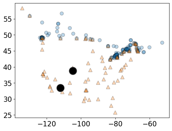
Let’s take 2 points (two feature vectors) from the cities dataset.

two_cities = X_cities.sample(2, random_state=120)
two_cities

	longitude	latitude
69	-104.8253	38.8340
35	-112.0741	33.4484

The two sampled points are shown as big black circles.

mglearn.discrete_scatter(
    X_cities.iloc[:, 0], X_cities.iloc[:, 1], y_cities, s=8, alpha=0.3
)
mglearn.discrete_scatter(
    two_cities.iloc[:, 0], two_cities.iloc[:, 1], markers="o", c="k", s=18
);

Distance between feature vectors

• For the cities at the two big circles, what is the distance between them?

• A common way to calculate the distance between vectors is calculating the Euclidean distance.

• The euclidean distance between vectors \(u = <u_1, u_2, \dots, u_n>\) and \(v = <v_1, v_2, \dots, v_n>\) is defined as:

\[distance(u, v) = \sqrt{\sum_{i =1}^{n} (u_i - v_i)^2}\]

Euclidean distance

two_cities

	longitude	latitude
69	-104.8253	38.8340
35	-112.0741	33.4484

• Subtract the two cities

• Square the difference

• Sum them up

• Take the square root

# Subtract the two cities
print("Subtract the cities: \n%s\n" % (two_cities.iloc[1] - two_cities.iloc[0]))

# Squared sum of the difference
print(
    "Sum of squares: %0.4f" % (np.sum((two_cities.iloc[1] - two_cities.iloc[0]) ** 2))
)

# Take the square root
print(
    "Euclidean distance between cities: %0.4f"
    % (np.sqrt(np.sum((two_cities.iloc[1] - two_cities.iloc[0]) ** 2)))
)

Subtract the cities: 
longitude   -7.2488
latitude    -5.3856
dtype: float64

Sum of squares: 81.5498
Euclidean distance between cities: 9.0305

two_cities

	longitude	latitude
69	-104.8253	38.8340
35	-112.0741	33.4484

# Euclidean distance using sklearn
from sklearn.metrics.pairwise import euclidean_distances

euclidean_distances(two_cities)

array([[0.        , 9.03049217],
       [9.03049217, 0.        ]])

Note: scikit-learn supports a number of other distance metrics.

Finding the nearest neighbour

• Let’s look at distances from all cities to all other cities

dists = euclidean_distances(X_cities)
np.fill_diagonal(dists, np.inf)
dists.shape

(209, 209)

pd.DataFrame(dists)

	0	1	2	3	4	5	6	7	8	9	...	199	200	201	202	203	204	205	206	207	208
0	inf	4.955113	9.869531	10.106452	10.449666	19.381676	28.366626	33.283857	33.572105	36.180388	...	9.834455	58.807684	16.925593	56.951696	59.384127	58.289799	64.183423	52.426410	58.033459	51.498562
1	4.955113	inf	14.677579	14.935802	15.305346	24.308448	33.200978	38.082949	38.359992	40.957919	...	14.668787	63.533498	21.656349	61.691640	64.045304	63.032656	68.887343	57.253724	62.771969	56.252160
2	9.869531	14.677579	inf	0.334411	0.808958	11.115406	20.528403	25.525757	25.873103	28.479109	...	0.277381	51.076798	10.783789	49.169693	51.934205	50.483751	56.512897	44.235152	50.249720	43.699224
3	10.106452	14.935802	0.334411	inf	0.474552	10.781004	20.194002	25.191396	25.538702	28.144750	...	0.275352	50.743133	10.480249	48.836189	51.599860	50.150395	56.179123	43.904226	49.916254	43.365623
4	10.449666	15.305346	0.808958	0.474552	inf	10.306500	19.719500	24.716985	25.064200	27.670344	...	0.675814	50.269880	10.051472	48.363192	51.125476	49.677629	55.705696	43.435186	49.443317	42.892477
...	...	...	...	...	...	...	...	...	...	...	...	...	...	...	...	...	...	...	...	...	...
204	58.289799	63.032656	50.483751	50.150395	49.677629	39.405415	30.043890	25.057003	24.746328	22.127878	...	50.333340	0.873356	41.380643	1.345136	3.373031	inf	6.102435	6.957987	0.316363	6.800190
205	64.183423	68.887343	56.512897	56.179123	55.705696	45.418031	36.031385	31.032874	30.709185	28.088948	...	56.358333	5.442806	47.259286	7.369875	5.108681	6.102435	inf	12.950733	6.303916	12.819584
206	52.426410	57.253724	44.235152	43.904226	43.435186	33.258427	24.059863	19.187663	18.932124	16.380495	...	44.100248	7.767852	35.637982	5.930561	9.731583	6.957987	12.950733	inf	6.837848	3.322755
207	58.033459	62.771969	50.249720	49.916254	49.443317	39.167214	29.799983	24.810368	24.497386	21.878183	...	50.098326	0.930123	41.121628	1.082749	3.286821	0.316363	6.303916	6.837848	inf	6.555740
208	51.498562	56.252160	43.699224	43.365623	42.892477	32.612755	23.244592	18.256813	17.946783	15.328953	...	43.546610	7.378764	34.596810	5.473691	8.568009	6.800190	12.819584	3.322755	6.555740	inf

209 rows × 209 columns

Let’s look at the distances between City 0 and some other cities.

print("Feature vector for city 0: \n%s\n" % (X_cities.iloc[0]))
print("Distances from city 0 to the first 5 cities: %s" % (dists[0][:5]))
# We can find the closest city with `np.argmin`:
print(
    "The closest city from city 0 is: %d \n\nwith feature vector: \n%s"
    % (np.argmin(dists[0]), X_cities.iloc[np.argmin(dists[0])])
)

Feature vector for city 0: 
longitude   -130.0437
latitude      55.9773
Name: 0, dtype: float64

Distances from city 0 to the first 5 cities: [        inf  4.95511263  9.869531   10.10645223 10.44966612]
The closest city from city 0 is: 81 

with feature vector: 
longitude   -129.9912
latitude      55.9383
Name: 81, dtype: float64

Ok, so the closest city to City 0 is City 81.

Question

• Why did we set the diagonal entries to infinity before finding the closest city?

Finding the distances to a query point

We can also find the distances to a new “test” or “query” city:

# Let's find a city that's closest to the a query city
query_point = [[-80, 25]]

dists = euclidean_distances(X_cities, query_point)
dists[0:10]

array([[58.85545875],
       [63.80062924],
       [49.30530902],
       [49.01473536],
       [48.60495488],
       [39.96834506],
       [32.92852376],
       [29.53520104],
       [29.52881619],
       [27.84679073]])

# The query point is closest to
print(
    "The query point %s is closest to the city with index %d and the distance between them is: %0.4f"
    % (query_point, np.argmin(dists), dists[np.argmin(dists)])
)

The query point [[-80, 25]] is closest to the city with index 72 and the distance between them is: 0.7982

\(k\)-Nearest Neighbours (\(k\)-NNs) [video]

small_cities = cities_df.sample(30, random_state=90)
one_city = small_cities.sample(1, random_state=44)
small_train_df = pd.concat([small_cities, one_city]).drop_duplicates(keep=False)

X_small_cities = small_train_df.drop(columns=["country"]).to_numpy()
y_small_cities = small_train_df["country"].to_numpy()
test_point = one_city[["longitude", "latitude"]].to_numpy()

plot_train_test_points(
    X_small_cities,
    y_small_cities,
    test_point,
    class_names=["Canada", "USA"],
    test_format="circle",
)

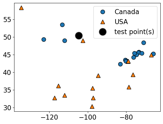
• Given a new data point, predict the class of the data point by finding the “closest” data point in the training set, i.e., by finding its “nearest neighbour” or majority vote of nearest neighbours.

Suppose we want to predict the class of the black point.

• An intuitive way to do this is predict the same label as the “closest” point (\(k = 1\)) (1-nearest neighbour)

• We would predict a target of USA in this case.

plot_knn_clf(
    X_small_cities,
    y_small_cities,
    test_point,
    n_neighbors=1,
    class_names=["Canada", "USA"],
    test_format="circle",
)

n_neighbors 1

How about using \(k > 1\) to get a more robust estimate?

• For example, we could also use the 3 closest points (k = 3) and let them vote on the correct class.

• The Canada class would win in this case.

plot_knn_clf(
    X_small_cities,
    y_small_cities,
    test_point,
    n_neighbors=3,
    class_names=["Canada", "USA"],
    test_format="circle",
)

n_neighbors 3

from sklearn.neighbors import KNeighborsClassifier

k_values = [1, 3]

for k in k_values:
    neigh = KNeighborsClassifier(n_neighbors=k)
    neigh.fit(X_small_cities, y_small_cities)
    print(
        "Prediction of the black dot with %d neighbours: %s"
        % (k, neigh.predict(test_point))
    )

Prediction of the black dot with 1 neighbours: ['USA']
Prediction of the black dot with 3 neighbours: ['Canada']

Choosing n_neighbors

• The primary hyperparameter of the model is n_neighbors (\(k\)) which decides how many neighbours should vote during prediction?

• What happens when we play around with n_neighbors?

• Are we more likely to overfit with a low n_neighbors or a high n_neighbors?

• Let’s examine the effect of the hyperparameter on our cities data.

X = cities_df.drop(columns=["country"])
y = cities_df["country"]

# split into train and test sets
X_train, X_test, y_train, y_test = train_test_split(
    X, y, test_size=0.1, random_state=123
)

k = 1
knn1 = KNeighborsClassifier(n_neighbors=k)
scores = cross_validate(knn1, X_train, y_train, return_train_score=True)
pd.DataFrame(scores)

	fit_time	score_time	test_score	train_score
0	0.001122	0.002389	0.710526	1.0
1	0.000835	0.001716	0.684211	1.0
2	0.000798	0.001676	0.842105	1.0
3	0.000790	0.001659	0.702703	1.0
4	0.000777	0.001647	0.837838	1.0

k = 100
knn100 = KNeighborsClassifier(n_neighbors=k)
scores = cross_validate(knn100, X_train, y_train, return_train_score=True)
pd.DataFrame(scores)

	fit_time	score_time	test_score	train_score
0	0.001025	0.048315	0.605263	0.600000
1	0.001002	0.002077	0.605263	0.600000
2	0.000807	0.002034	0.605263	0.600000
3	0.000809	0.001997	0.594595	0.602649
4	0.000795	0.001980	0.594595	0.602649

def f(n_neighbors=1):
    results = {}
    knn = KNeighborsClassifier(n_neighbors=n_neighbors)
    scores = cross_validate(knn, X_train, y_train, return_train_score=True)
    results["n_neighbours"] = [n_neighbors]
    results["mean_train_score"] = [round(scores["train_score"].mean(), 3)]
    results["mean_valid_score"] = [round(scores["test_score"].mean(), 3)]
    print(pd.DataFrame(results))


interactive(
    f,
    n_neighbors=widgets.IntSlider(min=1, max=101, step=5, value=1),
)

plot_knn_decision_boundaries(X_train, y_train, k_values=[1, 11, 100])

---------------------------------------------------------------------------
AttributeError                            Traceback (most recent call last)
File ~/miniconda3/envs/cpsc330/lib/python3.10/site-packages/mglearn/plot_2d_separator.py:86, in plot_2d_separator(classifier, X, fill, ax, eps, alpha, cm, linewidth, threshold, linestyle)
     85 try:
---> 86     decision_values = classifier.decision_function(X_grid)
     87     levels = [0] if threshold is None else [threshold]

AttributeError: 'KNeighborsClassifier' object has no attribute 'decision_function'

During handling of the above exception, another exception occurred:

KeyboardInterrupt                         Traceback (most recent call last)
Cell In[31], line 1
----> 1 plot_knn_decision_boundaries(X_train, y_train, k_values=[1, 11, 100])

File ~/CS/2023-24/330/cpsc330-2023W1/lectures/code/./plotting_functions.py:155, in plot_knn_decision_boundaries(X_train, y_train, k_values)
    153 mean_train_score = scores["train_score"].mean()
    154 clf.fit(X_train, y_train)
--> 155 mglearn.plots.plot_2d_separator(
    156     clf, X_train.to_numpy(), fill=True, eps=0.5, ax=ax, alpha=0.4
    157 )
    158 mglearn.discrete_scatter(X_train.iloc[:, 0], X_train.iloc[:, 1], y_train, ax=ax)
    159 title = "n_neighbors={}\n train score={}, valid score={}".format(
    160     n_neighbors, round(mean_train_score, 2), round(mean_valid_score, 2)
    161 )

File ~/miniconda3/envs/cpsc330/lib/python3.10/site-packages/mglearn/plot_2d_separator.py:92, in plot_2d_separator(classifier, X, fill, ax, eps, alpha, cm, linewidth, threshold, linestyle)
     88     fill_levels = [decision_values.min()] + levels + [
     89         decision_values.max()]
     90 except AttributeError:
     91     # no decision_function
---> 92     decision_values = classifier.predict_proba(X_grid)[:, 1]
     93     levels = [.5] if threshold is None else [threshold]
     94     fill_levels = [0] + levels + [1]

File ~/miniconda3/envs/cpsc330/lib/python3.10/site-packages/sklearn/neighbors/_classification.py:380, in KNeighborsClassifier.predict_proba(self, X)
    378 # a simple ':' index doesn't work right
    379 for i, idx in enumerate(pred_labels.T):  # loop is O(n_neighbors)
--> 380     proba_k[all_rows, idx] += weights[:, i]
    382 # normalize 'votes' into real [0,1] probabilities
    383 normalizer = proba_k.sum(axis=1)[:, np.newaxis]

KeyboardInterrupt: 

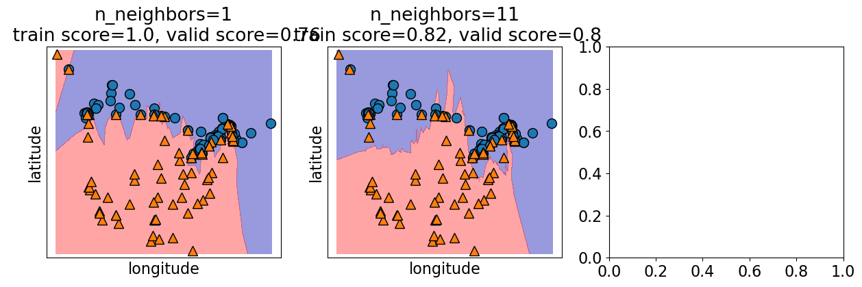
How to choose n_neighbors?

• n_neighbors is a hyperparameter

• We can use hyperparameter optimization to choose n_neighbors.

results_dict = {
    "n_neighbors": [],
    "mean_train_score": [],
    "mean_cv_score": [],
    "std_cv_score": [],
    "std_train_score": [],
}
param_grid = {"n_neighbors": np.arange(1, 50, 5)}

for k in param_grid["n_neighbors"]:
    knn = KNeighborsClassifier(n_neighbors=k)
    scores = cross_validate(knn, X_train, y_train, return_train_score=True)
    results_dict["n_neighbors"].append(k)

    results_dict["mean_cv_score"].append(np.mean(scores["test_score"]))
    results_dict["mean_train_score"].append(np.mean(scores["train_score"]))
    results_dict["std_cv_score"].append(scores["test_score"].std())
    results_dict["std_train_score"].append(scores["train_score"].std())

results_df = pd.DataFrame(results_dict)

results_df = results_df.set_index("n_neighbors")
results_df

	mean_train_score	mean_cv_score	std_cv_score	std_train_score
n_neighbors
1	1.000000	0.755477	0.069530	0.000000
6	0.831135	0.792603	0.046020	0.013433
11	0.819152	0.802987	0.041129	0.011336
16	0.801863	0.782219	0.074141	0.008735
21	0.777934	0.766430	0.062792	0.016944
26	0.755364	0.723613	0.061937	0.025910
31	0.743391	0.707681	0.057646	0.030408
36	0.728777	0.707681	0.064452	0.021305
41	0.706128	0.681223	0.061241	0.018310
46	0.694155	0.660171	0.093390	0.018178

results_df[["mean_train_score", "mean_cv_score"]].plot();

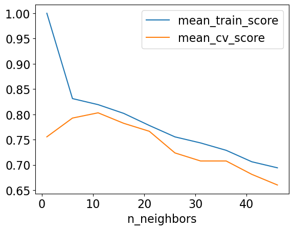
best_n_neighbours = results_df.idxmax()["mean_cv_score"]
best_n_neighbours

11

Let’s try our best model on test data.

knn = KNeighborsClassifier(n_neighbors=best_n_neighbours)
knn.fit(X_train, y_train)
print("Test accuracy: %0.3f" % (knn.score(X_test, y_test)))

Test accuracy: 0.905

Seems like we got lucky with the test set here.

❓❓ Questions for you

(iClicker) Exercise 3.1

iClicker cloud join link: https://join.iclicker.com/SNBF

Select all of the following statements which are TRUE.

• (A) Analogy-based models find examples from the test set that are most similar to the query example we are predicting.

• (B) Euclidean distance will always have a non-negative value.

• (C) With \(k\)-NN, setting the hyperparameter \(k\) to larger values typically reduces training error.

• (D) Similar to decision trees, \(k\)-NNs finds a small set of good features.

• (E) In \(k\)-NN, with \(k > 1\), the classification of the closest neighbour to the test example always contributes the most to the prediction.

Break (5 min)

More on \(k\)-NNs [video]

Other useful arguments of KNeighborsClassifier

• weights \(\rightarrow\) When predicting label, you can assign higher weight to the examples which are closer to the query example.

• Exercise for you: Play around with this argument. Do you get a better validation score?

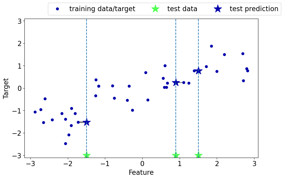
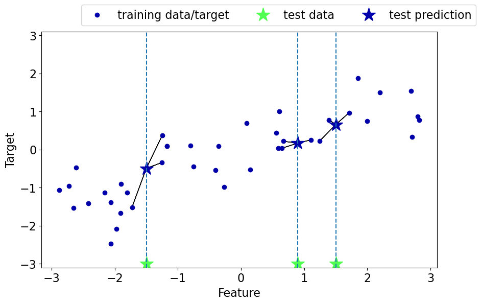
Regression with \(k\)-nearest neighbours (\(k\)-NNs)

• Can we solve regression problems with \(k\)-nearest neighbours algorithm?

• In \(k\)-NN regression we take the average of the \(k\)-nearest neighbours.

• We can also have weighted regression.

See an example of regression in the lecture notes.

mglearn.plots.plot_knn_regression(n_neighbors=1)

mglearn.plots.plot_knn_regression(n_neighbors=3)

Pros of \(k\)-NNs for supervised learning

• Easy to understand, interpret.

• Simple hyperparameter \(k\) (n_neighbors) controlling the fundamental tradeoff.

• Can learn very complex functions given enough data.

• Lazy learning: Takes no time to fit

Cons of \(k\)-NNs for supervised learning

• Can be potentially be VERY slow during prediction time, especially when the training set is very large.

• Often not that great test accuracy compared to the modern approaches.

• It does not work well on datasets with many features or where most feature values are 0 most of the time (sparse datasets).

Attention

For regular \(k\)-NN for supervised learning (not with sparse matrices), you should scale your features. We’ll be looking into it soon.

(Optional) Parametric vs non parametric

• You might see a lot of definitions of these terms.

• A simple way to think about this is:

  • do you need to store at least \(O(n)\) worth of stuff to make predictions? If so, it’s non-parametric.

• Non-parametric example: \(k\)-NN is a classic example of non-parametric models.

• Parametric example: decision stump

• If you want to know more about this, find some reading material here, here, and here.

• By the way, the terms “parametric” and “non-paramteric” are often used differently by statisticians, see here for more…

Note

\(\mathcal{O}(n)\) is referred to as big \(\mathcal{O}\) notation. It tells you how fast an algorithm is or how much storage space it requires. For example, in simple terms, if you have \(n\) examples and you need to store them all you can say that the algorithm requires \(\mathcal{O}(n)\) worth of stuff.

Curse of dimensionality

• Affects all learners but especially bad for nearest-neighbour.

• \(k\)-NN usually works well when the number of dimensions \(d\) is small but things fall apart quickly as \(d\) goes up.

• If there are many irrelevant attributes, \(k\)-NN is hopelessly confused because all of them contribute to finding similarity between examples.

• With enough irrelevant attributes the accidental similarity swamps out meaningful similarity and \(k\)-NN is no better than random guessing.

from sklearn.datasets import make_classification

nfeats_accuracy = {"nfeats": [], "dummy_valid_accuracy": [], "KNN_valid_accuracy": []}
for n_feats in range(4, 2000, 100):
    X, y = make_classification(n_samples=2000, n_features=n_feats, n_classes=2)
    X_train, X_test, y_train, y_test = train_test_split(
        X, y, test_size=0.2, random_state=123
    )
    dummy = DummyClassifier(strategy="most_frequent")
    dummy_scores = cross_validate(dummy, X_train, y_train, return_train_score=True)

    knn = KNeighborsClassifier()
    scores = cross_validate(knn, X_train, y_train, return_train_score=True)
    nfeats_accuracy["nfeats"].append(n_feats)
    nfeats_accuracy["KNN_valid_accuracy"].append(np.mean(scores["test_score"]))
    nfeats_accuracy["dummy_valid_accuracy"].append(np.mean(dummy_scores["test_score"]))

pd.DataFrame(nfeats_accuracy)

	nfeats	dummy_valid_accuracy	KNN_valid_accuracy
0	4	0.501875	0.946875
1	104	0.501875	0.769375
2	204	0.505000	0.653125
3	304	0.505000	0.633125
4	404	0.501250	0.682500
5	504	0.505625	0.620625
6	604	0.502500	0.662500
7	704	0.501250	0.636875
8	804	0.506250	0.579375
9	904	0.513750	0.590625
10	1004	0.503125	0.616875
11	1104	0.502500	0.617500
12	1204	0.510000	0.623125
13	1304	0.502500	0.635000
14	1404	0.504375	0.601875
15	1504	0.506250	0.588125
16	1604	0.506250	0.625625
17	1704	0.501250	0.572500
18	1804	0.508750	0.556250
19	1904	0.502500	0.590625

Support Vector Machines (SVMs) with RBF kernel [video]

• Very high-level overview

• Our goals here are

  • Use scikit-learn’s SVM model.

  • Broadly explain the notion of support vectors.

  • Broadly explain the similarities and differences between \(k\)-NNs and SVM RBFs.

  • Explain how C and gamma hyperparameters control the fundamental tradeoff.

(Optional) RBF stands for radial basis functions. We won’t go into what it means in this video. Refer to this video if you want to know more.

Overview

• Another popular similarity-based algorithm is Support Vector Machines with RBF Kernel (SVM RBFs)

• Superficially, SVM RBFs are more like weighted \(k\)-NNs.

  • The decision boundary is defined by a set of positive and negative examples and their weights together with their similarity measure.

  • A test example is labeled positive if on average it looks more like positive examples than the negative examples.

• The primary difference between \(k\)-NNs and SVM RBFs is that

  • Unlike \(k\)-NNs, SVM RBFs only remember the key examples (support vectors).

  • SVMs use a different similarity metric which is called a “kernel”. A popular kernel is Radial Basis Functions (RBFs)

  • They usually perform better than \(k\)-NNs!

Let’s explore SVM RBFs

Let’s try SVMs on the cities dataset.

mglearn.discrete_scatter(X_cities.iloc[:, 0], X_cities.iloc[:, 1], y_cities)
plt.xlabel("longitude")
plt.ylabel("latitude")
plt.legend(loc=1);

X_train, X_test, y_train, y_test = train_test_split(
    X_cities, y_cities, test_size=0.2, random_state=123
)

knn = KNeighborsClassifier(n_neighbors=best_n_neighbours)
scores = cross_validate(knn, X_train, y_train, return_train_score=True)
print("Mean validation score %0.3f" % (np.mean(scores["test_score"])))
pd.DataFrame(scores)

Mean validation score 0.803

	fit_time	score_time	test_score	train_score
0	0.001220	0.002158	0.794118	0.819549
1	0.001207	0.002132	0.764706	0.819549
2	0.001132	0.002036	0.727273	0.850746
3	0.003419	0.002297	0.787879	0.828358
4	0.001899	0.001910	0.939394	0.783582

from sklearn.svm import SVC

svm = SVC(gamma=0.01)  # Ignore gamma for now
scores = cross_validate(svm, X_train, y_train, return_train_score=True)
print("Mean validation score %0.3f" % (np.mean(scores["test_score"])))
pd.DataFrame(scores)

Mean validation score 0.820

	fit_time	score_time	test_score	train_score
0	0.005337	0.002172	0.823529	0.842105
1	0.001399	0.000810	0.823529	0.842105
2	0.001210	0.000763	0.727273	0.858209
3	0.001253	0.000789	0.787879	0.843284
4	0.001185	0.000767	0.939394	0.805970

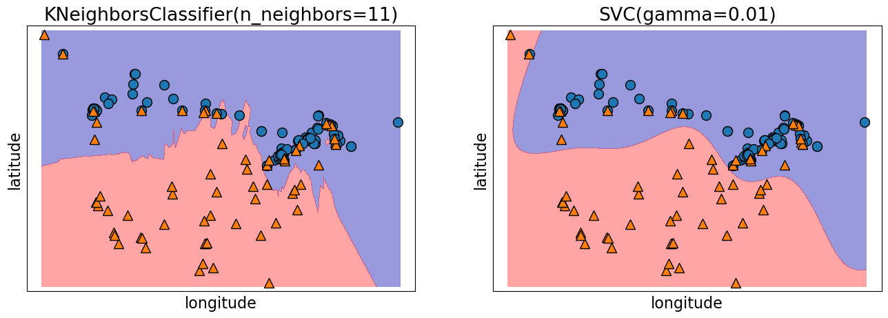
Decision boundary of SVMs

• We can think of SVM with RBF kernel as “smooth KNN”.

fig, axes = plt.subplots(1, 2, figsize=(16, 5))

for clf, ax in zip([knn, svm], axes):
    clf.fit(X_train, y_train)
    mglearn.plots.plot_2d_separator(
        clf, X_train.to_numpy(), fill=True, eps=0.5, ax=ax, alpha=0.4
    )
    mglearn.discrete_scatter(X_train.iloc[:, 0], X_train.iloc[:, 1], y_train, ax=ax)
    ax.set_title(clf)
    ax.set_xlabel("longitude")
    ax.set_ylabel("latitude")

Support vectors

• Each training example either is or isn’t a “support vector”.

  • This gets decided during fit.

• Main insight: the decision boundary only depends on the support vectors.

• Let’s look at the support vectors.

from sklearn.datasets import make_blobs

n = 20
n_classes = 2
X_toy, y_toy = make_blobs(
    n_samples=n, centers=n_classes, random_state=300
)  # Let's generate some fake data

mglearn.discrete_scatter(X_toy[:, 0], X_toy[:, 1], y_toy)
plt.xlabel("Feature 0")
plt.ylabel("Feature 1")
svm = SVC(kernel="rbf", C=10, gamma=0.1).fit(X_toy, y_toy)
mglearn.plots.plot_2d_separator(svm, X_toy, fill=True, eps=0.5, alpha=0.4)

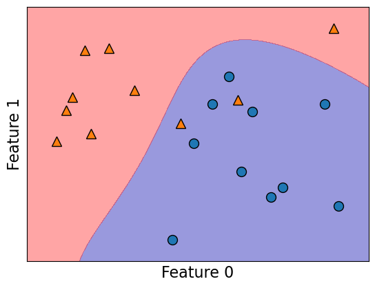
svm.support_

array([ 3,  8,  9, 14, 19,  1,  4,  6, 17], dtype=int32)

plot_support_vectors(svm, X_toy, y_toy)

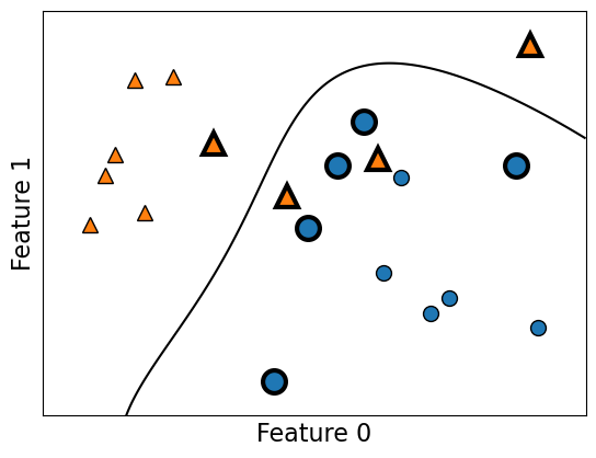
The support vectors are the bigger points in the plot above.

Hyperparameters of SVM

• Key hyperparameters of rbf SVM are

  • gamma

  • C

• We are not equipped to understand the meaning of these parameters at this point but you are expected to describe their relation to the fundamental tradeoff.

See scikit-learn’s explanation of RBF SVM parameters.

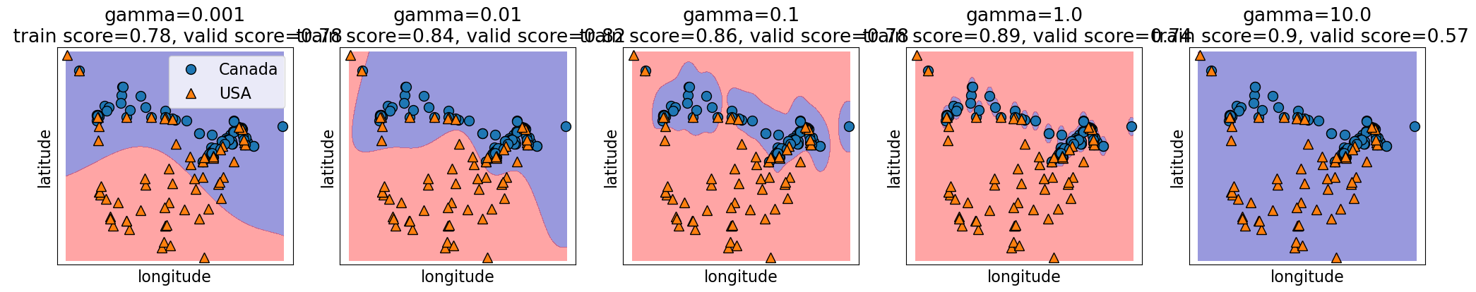
Relation of gamma and the fundamental trade-off

• gamma controls the complexity (fundamental trade-off), just like other hyperparameters we’ve seen.

  • larger gamma \(\rightarrow\) more complex

  • smaller gamma \(\rightarrow\) less complex

gamma = [0.001, 0.01, 0.1, 1.0, 10.0]
plot_svc_gamma(
    gamma,
    X_train.to_numpy(),
    y_train.to_numpy(),
    x_label="longitude",
    y_label="latitude",
)

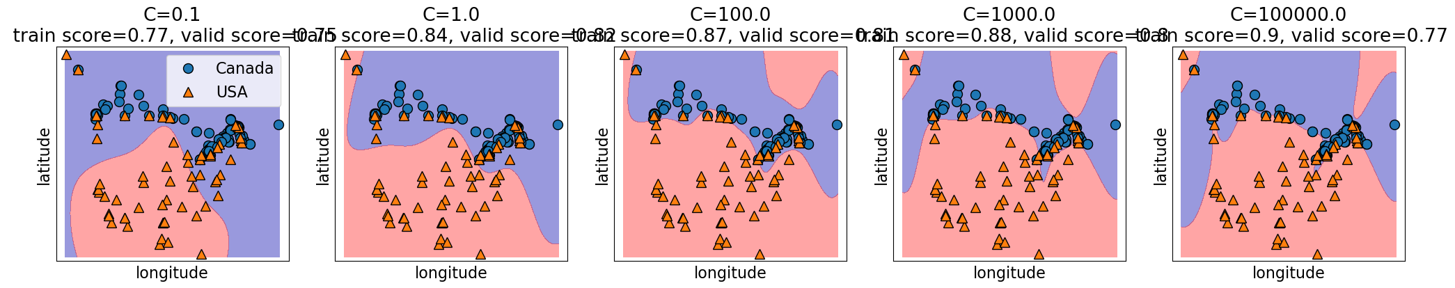
Relation of C and the fundamental trade-off

• C also affects the fundamental tradeoff

  • larger C \(\rightarrow\) more complex

  • smaller C \(\rightarrow\) less complex

C = [0.1, 1.0, 100.0, 1000.0, 100000.0]
plot_svc_C(
    C, X_train.to_numpy(), y_train.to_numpy(), x_label="longitude", y_label="latitude"
)

Search over multiple hyperparameters

• So far you have seen how to carry out search over a hyperparameter

• In the above case the best training error is achieved by the most complex model (large gamma, large C).

• Best validation error requires a hyperparameter search to balance the fundamental tradeoff.

  • In general we can’t search them one at a time.

  • More on this next week. But if you cannot wait till then, you may look up the following:

    • sklearn.model_selection.GridSearchCV

    • sklearn.model_selection.RandomizedSearchCV

SVM Regressor

• Similar to KNNs, you can use SVMs for regression problems as well.

• See sklearn.svm.SVR for more details.

❓❓ Questions for you

(iClicker) Exercise 3.2

iClicker cloud join link: https://join.iclicker.com/SNBF

Select all of the following statements which are TRUE.

• (A) \(k\)-NN may perform poorly in high-dimensional space (say, d > 1000).

• (B) In SVM RBF, removing a non-support vector would not change the decision boundary.

• (C) In sklearn’s SVC classifier, large values of gamma tend to result in higher training score but probably lower validation score.

• (D) If we increase both gamma and C, we can’t be certain if the model becomes more complex or less complex.

More practice questions

• Check out some more practice questions here.

Summary

• We have KNNs and SVMs as new supervised learning techniques in our toolbox.

• These are analogy-based learners and the idea is to assign nearby points the same label.

• Unlike decision trees, all features are equally important.

• Both can be used for classification or regression (much like the other methods we’ve seen).

Coming up:

Lingering questions:

• Are we ready to do machine learning on real-world datasets?

• What would happen if we use \(k\)-NNs or SVM RBFs on the spotify dataset from hw1?

• What happens if we have missing values in our data?

• What do we do if we have features with categories or string values?