Lecture 20: Survival analysis

UBC 2023-24

Instructor: Varada Kolhatkar and Andrew Roth

Imports

import matplotlib.pyplot as plt
import numpy as np

import pandas as pd
from sklearn.compose import ColumnTransformer, make_column_transformer
from sklearn.dummy import DummyClassifier
from sklearn.ensemble import RandomForestClassifier, RandomForestRegressor
from sklearn.impute import SimpleImputer
from sklearn.linear_model import LogisticRegression, Ridge
from sklearn.metrics import confusion_matrix
from sklearn.model_selection import (
    cross_val_predict,
    cross_val_score,
    cross_validate,
    train_test_split,
)
from sklearn.pipeline import Pipeline, make_pipeline
from sklearn.preprocessing import (
    FunctionTransformer,
    OneHotEncoder,
    OrdinalEncoder,
    StandardScaler,
)
import sys
import os

sys.path.append(os.path.join(os.path.abspath("."), "code"))
from utils import *

plt.rcParams["font.size"] = 12

# does lifelines try to mess with this?
pd.options.display.max_rows = 10

import warnings
warnings.filterwarnings('default')

import lifelines

---------------------------------------------------------------------------
ModuleNotFoundError                       Traceback (most recent call last)
Cell In[2], line 1
----> 1 import lifelines

ModuleNotFoundError: No module named 'lifelines'

Learning objectives

• Explain what is right-censored data.

• Explain the problem with treating right-censored data the same as “regular” data.

• Determine whether survival analysis is an appropriate tool for a given problem.

• Apply survival analysis in Python using the lifelines package.

• Interpret a survival curve, such as the Kaplan-Meier curve.

• Interpret the coefficients of a fitted Cox proportional hazards model.

• Make predictions for existing individuals and interpret these predictions.

❓❓ Questions for you

(iClicker) Exercise 20.1

iClicker cloud join link: https://join.iclicker.com/SNBF

Select all of the following statements which are TRUE.

• (A) We need to be careful when splitting the data when working with time series data.

• (B) Cross-validation in time series can be randomly applied like in other machine learning tasks.

• (C) In time series forecasting, the future value of a series can only be predicted based on its past values and cannot incorporate other variables.

• (D) When we used RandomForestRegressor model on the POSIX time feature, it predicted a straight line on the test data because tree-based models are inherently unable to extrapolate (i.e., make predictions outside the range of the training data).
  
  
  
  

Recap

• Time series analysis is used when there is a temporal aspect in the data.

• Data splitting: Data should be split based on time to avoid future data leaking into the training set.

• Essential questions for Exploratory Data Analysis (EDA):

  • What is the frequency of data collection (e.g., hourly, daily)?

  • How many time series are present within the dataset?

  • Are there any gaps or missing values in the data?

• Feature engineering

  • Derived new features from the date/time column.

  • Appropriately encoded features based on the chosen model.

  • Created lag features to incorporate past values for prediction.

• Baseline model approach: Employ a simple model, such as using today’s target value to predict tomorrow’s, as a starting point for comparison.

• Cross-Validation Method for Time Series: In sklearn, use TimeSeriesSplit as the cv parameter in functions like cross_validate or cross_val_score for time-appropriate validation.

• Strategies for long-term forecasting:

  • Generate forecasts for sequential time steps by assuming the predictions for the previous steps are accurate.

• Trends

  • A ‘days since’ feature to capture the trend over time

Customer churn

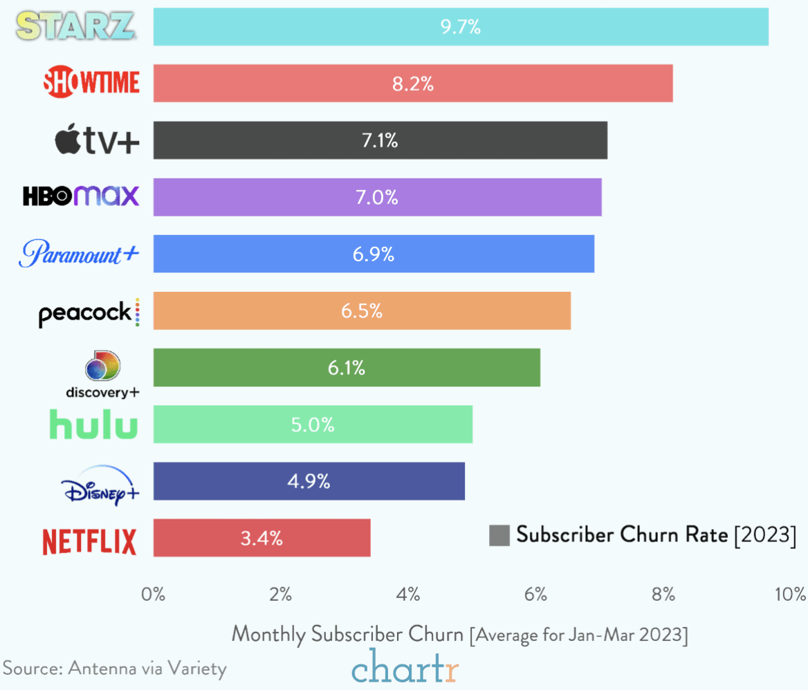
• Customer churn, also known as customer attrition, refers to the phenomenon where customers or subscribers stop doing business with a company or service.

• The bar-chart below is showing the monthly subscriber churn rates for various streaming services.

• Imagine that you are working for a subscription-based telecom company.

• They want to predict when a specific customer will churn so that they can come up with retention strategies for different customer segments.

• We want to model “time to churn” to understand different factors affecting customer churn.

• Is it possible to use machine learning to predict whether a specific customer will churn?

Let’s work with this dataset Customer Churn Dataset, which is collected at a fixed time.

df = pd.read_csv("data/WA_Fn-UseC_-Telco-Customer-Churn.csv")
train_df, test_df = train_test_split(df, random_state=123)
train_df.head()

	customerID	gender	SeniorCitizen	Partner	Dependents	tenure	PhoneService	MultipleLines	InternetService	OnlineSecurity	...	DeviceProtection	TechSupport	StreamingTV	StreamingMovies	Contract	PaperlessBilling	PaymentMethod	MonthlyCharges	TotalCharges	Churn
6464	4726-DLWQN	Male	1	No	No	50	Yes	Yes	DSL	Yes	...	No	No	Yes	No	Month-to-month	Yes	Bank transfer (automatic)	70.35	3454.6	No
5707	4537-DKTAL	Female	0	No	No	2	Yes	No	DSL	No	...	No	No	No	No	Month-to-month	No	Electronic check	45.55	84.4	No
3442	0468-YRPXN	Male	0	No	No	29	Yes	No	Fiber optic	No	...	Yes	Yes	Yes	Yes	Month-to-month	Yes	Credit card (automatic)	98.80	2807.1	No
3932	1304-NECVQ	Female	1	No	No	2	Yes	Yes	Fiber optic	No	...	Yes	No	No	No	Month-to-month	Yes	Electronic check	78.55	149.55	Yes
6124	7153-CHRBV	Female	0	Yes	Yes	57	Yes	No	DSL	Yes	...	Yes	Yes	No	No	One year	Yes	Mailed check	59.30	3274.35	No

5 rows × 21 columns

• We are interested in predicting customer churn: the “Churn” column.

• How will you approach this problem with the approaches we have seen so far?

• How about treating this as a binary classification problem where we want to predict Churn (yes/no) from these -other columns.

• Before we look into survival analysis, let’s just treat it as a binary classification model where we want to predict whether a customer churned or not.

train_df.shape

(5282, 21)

train_df["Churn"].value_counts()

Churn
No     3912
Yes    1370
Name: count, dtype: int64

train_df.info()

<class 'pandas.core.frame.DataFrame'>
Index: 5282 entries, 6464 to 3582
Data columns (total 21 columns):
 #   Column            Non-Null Count  Dtype  
---  ------            --------------  -----  
 0   customerID        5282 non-null   object 
 1   gender            5282 non-null   object 
 2   SeniorCitizen     5282 non-null   int64  
 3   Partner           5282 non-null   object 
 4   Dependents        5282 non-null   object 
 5   tenure            5282 non-null   int64  
 6   PhoneService      5282 non-null   object 
 7   MultipleLines     5282 non-null   object 
 8   InternetService   5282 non-null   object 
 9   OnlineSecurity    5282 non-null   object 
 10  OnlineBackup      5282 non-null   object 
 11  DeviceProtection  5282 non-null   object 
 12  TechSupport       5282 non-null   object 
 13  StreamingTV       5282 non-null   object 
 14  StreamingMovies   5282 non-null   object 
 15  Contract          5282 non-null   object 
 16  PaperlessBilling  5282 non-null   object 
 17  PaymentMethod     5282 non-null   object 
 18  MonthlyCharges    5282 non-null   float64
 19  TotalCharges      5282 non-null   object 
 20  Churn             5282 non-null   object 
dtypes: float64(1), int64(2), object(18)
memory usage: 907.8+ KB

Question: Does this mean there is no missing data?

Ok, let’s try our usual approach:

train_df["SeniorCitizen"].value_counts()

SeniorCitizen
0    4430
1     852
Name: count, dtype: int64

numeric_features = ["tenure", "MonthlyCharges", "TotalCharges"]
drop_features = ["customerID"]
passthrough_features = ["SeniorCitizen"]
target_column = ["Churn"]
# the rest are categorical
categorical_features = list(
    set(train_df.columns)
    - set(numeric_features)
    - set(passthrough_features)
    - set(drop_features)
    - set(target_column)
)

preprocessor = make_column_transformer(
    (StandardScaler(), numeric_features),
    (OneHotEncoder(), categorical_features),
    ("passthrough", passthrough_features),
    ("drop", drop_features),
)

# preprocessor.fit(train_df);

Hmmm, one of the numeric features is causing problems?

df.info()

<class 'pandas.core.frame.DataFrame'>
RangeIndex: 7043 entries, 0 to 7042
Data columns (total 21 columns):
 #   Column            Non-Null Count  Dtype  
---  ------            --------------  -----  
 0   customerID        7043 non-null   object 
 1   gender            7043 non-null   object 
 2   SeniorCitizen     7043 non-null   int64  
 3   Partner           7043 non-null   object 
 4   Dependents        7043 non-null   object 
 5   tenure            7043 non-null   int64  
 6   PhoneService      7043 non-null   object 
 7   MultipleLines     7043 non-null   object 
 8   InternetService   7043 non-null   object 
 9   OnlineSecurity    7043 non-null   object 
 10  OnlineBackup      7043 non-null   object 
 11  DeviceProtection  7043 non-null   object 
 12  TechSupport       7043 non-null   object 
 13  StreamingTV       7043 non-null   object 
 14  StreamingMovies   7043 non-null   object 
 15  Contract          7043 non-null   object 
 16  PaperlessBilling  7043 non-null   object 
 17  PaymentMethod     7043 non-null   object 
 18  MonthlyCharges    7043 non-null   float64
 19  TotalCharges      7043 non-null   object 
 20  Churn             7043 non-null   object 
dtypes: float64(1), int64(2), object(18)
memory usage: 1.1+ MB

Oh, looks like TotalCharges is not a numeric type. What if we change the type of this column to float?

train_df["TotalCharges"] = train_df["TotalCharges"].astype(float)

---------------------------------------------------------------------------
ValueError                                Traceback (most recent call last)
Cell In[12], line 1
----> 1 train_df["TotalCharges"] = train_df["TotalCharges"].astype(float)

File ~/miniconda3/envs/cpsc330/lib/python3.10/site-packages/pandas/core/generic.py:6534, in NDFrame.astype(self, dtype, copy, errors)
   6530     results = [ser.astype(dtype, copy=copy) for _, ser in self.items()]
   6532 else:
   6533     # else, only a single dtype is given
-> 6534     new_data = self._mgr.astype(dtype=dtype, copy=copy, errors=errors)
   6535     res = self._constructor_from_mgr(new_data, axes=new_data.axes)
   6536     return res.__finalize__(self, method="astype")

File ~/miniconda3/envs/cpsc330/lib/python3.10/site-packages/pandas/core/internals/managers.py:414, in BaseBlockManager.astype(self, dtype, copy, errors)
    411 elif using_copy_on_write():
    412     copy = False
--> 414 return self.apply(
    415     "astype",
    416     dtype=dtype,
    417     copy=copy,
    418     errors=errors,
    419     using_cow=using_copy_on_write(),
    420 )

File ~/miniconda3/envs/cpsc330/lib/python3.10/site-packages/pandas/core/internals/managers.py:354, in BaseBlockManager.apply(self, f, align_keys, **kwargs)
    352         applied = b.apply(f, **kwargs)
    353     else:
--> 354         applied = getattr(b, f)(**kwargs)
    355     result_blocks = extend_blocks(applied, result_blocks)
    357 out = type(self).from_blocks(result_blocks, self.axes)

File ~/miniconda3/envs/cpsc330/lib/python3.10/site-packages/pandas/core/internals/blocks.py:616, in Block.astype(self, dtype, copy, errors, using_cow)
    596 """
    597 Coerce to the new dtype.
    598 
   (...)
    612 Block
    613 """
    614 values = self.values
--> 616 new_values = astype_array_safe(values, dtype, copy=copy, errors=errors)
    618 new_values = maybe_coerce_values(new_values)
    620 refs = None

File ~/miniconda3/envs/cpsc330/lib/python3.10/site-packages/pandas/core/dtypes/astype.py:238, in astype_array_safe(values, dtype, copy, errors)
    235     dtype = dtype.numpy_dtype
    237 try:
--> 238     new_values = astype_array(values, dtype, copy=copy)
    239 except (ValueError, TypeError):
    240     # e.g. _astype_nansafe can fail on object-dtype of strings
    241     #  trying to convert to float
    242     if errors == "ignore":

File ~/miniconda3/envs/cpsc330/lib/python3.10/site-packages/pandas/core/dtypes/astype.py:183, in astype_array(values, dtype, copy)
    180     values = values.astype(dtype, copy=copy)
    182 else:
--> 183     values = _astype_nansafe(values, dtype, copy=copy)
    185 # in pandas we don't store numpy str dtypes, so convert to object
    186 if isinstance(dtype, np.dtype) and issubclass(values.dtype.type, str):

File ~/miniconda3/envs/cpsc330/lib/python3.10/site-packages/pandas/core/dtypes/astype.py:134, in _astype_nansafe(arr, dtype, copy, skipna)
    130     raise ValueError(msg)
    132 if copy or arr.dtype == object or dtype == object:
    133     # Explicit copy, or required since NumPy can't view from / to object.
--> 134     return arr.astype(dtype, copy=True)
    136 return arr.astype(dtype, copy=copy)

ValueError: could not convert string to float: ''

Argh!!

for val in train_df["TotalCharges"]:
    try:
        float(val)
    except ValueError:
        print(val)

Any ideas?

Well, it turns out we can’t see those problematic values because they are whitespace!

for val in train_df["TotalCharges"]:
    try:
        float(val)
    except ValueError:
        print('"%s"' % val)

" "
" "
" "
" "
" "
" "
" "
" "

Let’s replace the whitespaces with NaNs.

train_df = train_df.assign(
    TotalCharges=train_df["TotalCharges"].replace(" ", np.nan).astype(float)
)
test_df = test_df.assign(
    TotalCharges=test_df["TotalCharges"].replace(" ", np.nan).astype(float)
)

train_df.info()

<class 'pandas.core.frame.DataFrame'>
Index: 5282 entries, 6464 to 3582
Data columns (total 21 columns):
 #   Column            Non-Null Count  Dtype  
---  ------            --------------  -----  
 0   customerID        5282 non-null   object 
 1   gender            5282 non-null   object 
 2   SeniorCitizen     5282 non-null   int64  
 3   Partner           5282 non-null   object 
 4   Dependents        5282 non-null   object 
 5   tenure            5282 non-null   int64  
 6   PhoneService      5282 non-null   object 
 7   MultipleLines     5282 non-null   object 
 8   InternetService   5282 non-null   object 
 9   OnlineSecurity    5282 non-null   object 
 10  OnlineBackup      5282 non-null   object 
 11  DeviceProtection  5282 non-null   object 
 12  TechSupport       5282 non-null   object 
 13  StreamingTV       5282 non-null   object 
 14  StreamingMovies   5282 non-null   object 
 15  Contract          5282 non-null   object 
 16  PaperlessBilling  5282 non-null   object 
 17  PaymentMethod     5282 non-null   object 
 18  MonthlyCharges    5282 non-null   float64
 19  TotalCharges      5274 non-null   float64
 20  Churn             5282 non-null   object 
dtypes: float64(2), int64(2), object(17)
memory usage: 907.8+ KB

But now we are going to have missing values and we need to include imputation for numeric features in our preprocessor.

preprocessor = make_column_transformer(
    (
        make_pipeline(SimpleImputer(strategy="median"), StandardScaler()),
        numeric_features,
    ),
    (OneHotEncoder(handle_unknown="ignore"), categorical_features),
    ("passthrough", passthrough_features),
    ("drop", drop_features),
)

Now let’s try that again…

preprocessor.fit(train_df);

It worked! Let’s get the column names of the transformed data from the column transformer.

new_columns = (
    numeric_features
    + preprocessor.named_transformers_["onehotencoder"]
    .get_feature_names_out(categorical_features)
    .tolist()
    + passthrough_features
)

X_train_enc = pd.DataFrame(
    preprocessor.transform(train_df), index=train_df.index, columns=new_columns
)
X_test_enc = pd.DataFrame(
    preprocessor.transform(train_df), index=train_df.index, columns=new_columns
)

X_train_enc.head()

	tenure	MonthlyCharges	TotalCharges	MultipleLines_No	MultipleLines_No phone service	MultipleLines_Yes	gender_Female	gender_Male	PaymentMethod_Bank transfer (automatic)	PaymentMethod_Credit card (automatic)	...	OnlineSecurity_No internet service	OnlineSecurity_Yes	PhoneService_No	PhoneService_Yes	DeviceProtection_No	DeviceProtection_No internet service	DeviceProtection_Yes	Dependents_No	Dependents_Yes	SeniorCitizen
6464	0.707712	0.185175	0.513678	0.0	0.0	1.0	0.0	1.0	1.0	0.0	...	0.0	1.0	0.0	1.0	1.0	0.0	0.0	1.0	0.0	1.0
5707	-1.248999	-0.641538	-0.979562	1.0	0.0	0.0	1.0	0.0	0.0	0.0	...	0.0	0.0	0.0	1.0	1.0	0.0	0.0	1.0	0.0	0.0
3442	-0.148349	1.133562	0.226789	1.0	0.0	0.0	0.0	1.0	0.0	1.0	...	0.0	0.0	0.0	1.0	0.0	0.0	1.0	1.0	0.0	0.0
3932	-1.248999	0.458524	-0.950696	0.0	0.0	1.0	1.0	0.0	0.0	0.0	...	0.0	0.0	0.0	1.0	0.0	0.0	1.0	1.0	0.0	1.0
6124	0.993065	-0.183179	0.433814	1.0	0.0	0.0	1.0	0.0	0.0	0.0	...	0.0	1.0	0.0	1.0	0.0	0.0	1.0	0.0	1.0	0.0

5 rows × 45 columns

results = {}

X_train = train_df.drop(columns=["Churn"])
X_test = test_df.drop(columns=["Churn"])

y_train = train_df["Churn"]
y_test = test_df["Churn"]

DummyClassifier

dc = DummyClassifier()

results["dummy"] = mean_std_cross_val_scores(
    dc, X_train, y_train, return_train_score=True
)
pd.DataFrame(results).T

	fit_time	score_time	test_score	train_score
dummy	0.002 (+/- 0.000)	0.002 (+/- 0.000)	0.741 (+/- 0.000)	0.741 (+/- 0.000)

Dummy model scores are pretty good because we have class imbalance.

y_train.value_counts()

Churn
No     3912
Yes    1370
Name: count, dtype: int64

LogisticRegression

lr = make_pipeline(preprocessor, LogisticRegression(max_iter=1000))

results["logistic regression"] = mean_std_cross_val_scores(
    lr, X_train, y_train, return_train_score=True
)
pd.DataFrame(results).T

	fit_time	score_time	test_score	train_score
dummy	0.002 (+/- 0.000)	0.002 (+/- 0.000)	0.741 (+/- 0.000)	0.741 (+/- 0.000)
logistic regression	0.047 (+/- 0.004)	0.006 (+/- 0.000)	0.804 (+/- 0.013)	0.809 (+/- 0.002)

confusion_matrix(y_train, cross_val_predict(lr, X_train, y_train))

array([[3516,  396],
       [ 637,  733]])

• Logistic regression beats the dummy model.

• But it seems like we have many false negatives.

RandomForestClassifier

Let’s try random forest model.

rf = make_pipeline(preprocessor, RandomForestClassifier(n_estimators=100))

results["random forest"] = mean_std_cross_val_scores(
    rf, X_train, y_train, return_train_score=True
)
pd.DataFrame(results).T

	fit_time	score_time	test_score	train_score
dummy	0.002 (+/- 0.000)	0.002 (+/- 0.000)	0.741 (+/- 0.000)	0.741 (+/- 0.000)
logistic regression	0.047 (+/- 0.004)	0.006 (+/- 0.000)	0.804 (+/- 0.013)	0.809 (+/- 0.002)
random forest	0.329 (+/- 0.012)	0.019 (+/- 0.001)	0.790 (+/- 0.013)	0.998 (+/- 0.000)

confusion_matrix(y_train, cross_val_predict(rf, X_train, y_train))

array([[3518,  394],
       [ 743,  627]])

• Random forest is not improving the scores.

• We might decide to do hyperparamter optimization to further improve the score.

• But after trying out all the usual things should we be happy with the scores?

• Are we doing anything fundamentally wrong when we treat this problem as a binary classification?
  
  
  
  
  
  
  

The rest of the class is about what is wrong with what we just did!

Censoring and survival analysis

Time to event and censoring

• When we treat the problem as a binary classification problem, we predict whether a customer would churn or not at a particular point in time, when the data was collected.

• If a customer has not churned yet, wouldn’t it be more useful to understand when they are likely to churn so that we can offer them promotions etc?

• Here we are actually interested in the time till the event of churn occurs.

There are many situations where you want to analyze the time until an event occurs. For example,

• the time until a customer leaves a subscription service (this dataset)

• the time until a disease kills its host

• the time until a piece of equipment breaks

• the time that someone unemployed will take to land a new job

• the time until you wait for your turn to get a surgery

Although this branch of statistics is usually referred to as Survival Analysis, the event in question does not need to be related to actual “survival”. The important thing is to understand that we are interested in the time until something happens, or whether or not something will happen in a certain time frame.

In our dataset there is a column called “tenure”, which encodes this temporal aspect of the data.

train_df[["tenure"]].head()

	tenure
6464	50
5707	2
3442	29
3932	2
6124	57

• The tenure column is the number of months the customer has stayed with the company.

• But we only have information about this till the point we collected the data.

❓❓ Questions for you

But why is this different? Can’t you just use the techniques you learned so far (e.g., regression models) to predict the time (tenure in our case)? Take a minute to think about this. What could be possible scenarios for the duration column?

The answer would be yes if you could observe the actual time in all occurrences, but you usually cannot. Frequently, there will be some kind of censoring which will not allow you to observe the exact time that the event happened for all units/individuals that are being studied.

train_df[["tenure", "Churn"]].head()

	tenure	Churn
6464	50	No
5707	2	No
3442	29	No
3932	2	Yes
6124	57	No

• What this means is that we don’t have correct target values to train or test our model.

• This is a problem!

Let’s consider some approaches to deal with this censoring issue.

Approach 1: Only consider the examples where “Churn”=Yes

Let’s just consider the cases for which we have the time, to obtain the average subscription length.

train_df_churn = train_df.query(
    "Churn == 'Yes'"
)  # Consider only examples where the customers churned.
test_df_churn = test_df.query(
    "Churn == 'Yes'"
)  # Consider only examples where the customers churned.
train_df_churn.head()

	customerID	gender	SeniorCitizen	Partner	Dependents	tenure	PhoneService	MultipleLines	InternetService	OnlineSecurity	...	DeviceProtection	TechSupport	StreamingTV	StreamingMovies	Contract	PaperlessBilling	PaymentMethod	MonthlyCharges	TotalCharges	Churn
3932	1304-NECVQ	Female	1	No	No	2	Yes	Yes	Fiber optic	No	...	Yes	No	No	No	Month-to-month	Yes	Electronic check	78.55	149.55	Yes
301	8098-LLAZX	Female	1	No	No	4	Yes	Yes	Fiber optic	No	...	No	No	Yes	Yes	Month-to-month	Yes	Electronic check	95.45	396.10	Yes
5540	3803-KMQFW	Female	0	Yes	Yes	1	Yes	No	No	No internet service	...	No internet service	No internet service	No internet service	No internet service	Month-to-month	No	Mailed check	20.55	20.55	Yes
4084	2777-PHDEI	Female	0	No	No	1	Yes	No	Fiber optic	No	...	No	No	Yes	No	Month-to-month	No	Electronic check	78.05	78.05	Yes
3272	6772-KSATR	Male	0	No	No	1	Yes	Yes	Fiber optic	Yes	...	No	No	No	No	Month-to-month	Yes	Electronic check	81.70	81.70	Yes

5 rows × 21 columns

train_df.shape

(5282, 21)

train_df_churn.shape

(1370, 21)

numeric_features

['tenure', 'MonthlyCharges', 'TotalCharges']

preprocessing_notenure = make_column_transformer(
    (
        make_pipeline(SimpleImputer(strategy="median"), StandardScaler()),
        numeric_features[1:],  # Getting rid of the tenure column
    ),
    (OneHotEncoder(handle_unknown="ignore"), categorical_features),
    ("passthrough", passthrough_features),
)

tenure_lm = make_pipeline(preprocessing_notenure, Ridge())

tenure_lm.fit(train_df_churn.drop(columns=["tenure"]), train_df_churn["tenure"]);

pd.DataFrame(
    tenure_lm.predict(test_df_churn.drop(columns=["tenure"]))[:10],
    columns=["tenure_predictions"],
)

	tenure_predictions
0	5.062449
1	13.198645
2	11.859455
3	5.865562
4	58.154842
5	3.757932
6	18.932070
7	7.720893
8	36.818041
9	7.263541

❓❓ Questions for you

What will be wrong with our estimated survival times? Will they be too low or too high?

On average they will be underestimates (too small), because we are ignoring the currently subscribed (un-churned) customers. Our dataset is a biased sample of those who churned within the time window of the data collection. Long-time subscribers were more likely to be removed from the dataset! This is a common mistake - see the Calling Bullshit video from the README!

Approach 2: Assume everyone churns right now

Assume everyone churns right now - in other words, use the original dataset.

train_df[["tenure", "Churn"]].head()

	tenure	Churn
6464	50	No
5707	2	No
3442	29	No
3932	2	Yes
6124	57	No

tenure_lm.fit(train_df.drop(columns=["tenure"]), train_df["tenure"]);

pd.DataFrame(
    tenure_lm.predict(test_df_churn.drop(columns=["tenure"]))[:10],
    columns=["tenure_predictions"],
)

	tenure_predictions
0	6.400047
1	20.220392
2	22.332746
3	12.825470
4	59.885968
5	7.075453
6	17.731498
7	10.407862
8	38.425365
9	10.854500

❓❓ Questions for you

What will be wrong with our estimated survival time?

train_df[["tenure", "Churn"]].head()

	tenure	Churn
6464	50	No
5707	2	No
3442	29	No
3932	2	Yes
6124	57	No

It will be an underestimate again. For those still subscribed, while we did not remove them, we recorded a total tenure shorter than in reality, because they will keep going for some amount of time.

Approach 3: Survival analysis

Deal with this properly using survival analysis.

• You may learn about this in a statistics course.

• We will use the lifelines package in Python and will not go into the math/stats of how it works.

train_df[["tenure", "Churn"]].head()

	tenure	Churn
6464	50	No
5707	2	No
3442	29	No
3932	2	Yes
6124	57	No

Types of questions we might want to answer:

1. How long do customers stay with the service?

2. For a particular customer, can we predict how long they might stay with the service?

3. What factors influence a customer’s churn time?

Break (5 min)

❓❓ Questions for you

(iClicker) Exercise 20.2

iClicker cloud join link: https://join.iclicker.com/SNBF

Select all of the following statements which are TRUE.

• (A) Right censoring occurs when the endpoint of event has not been observed for all study subjects by the end of the study period.

• (B) Right censoring implies that the data is missing completely at random.

• (C) In the presence of right-censored data, binary classification models can be applied directly without any modifications or special considerations.

• (D) If we apply the Ridge regression model to predict tenure in right censored data, we are likely to underestimate it because the tenure observed in our data is shorter than what it would be in reality.

Kaplan-Meier survival curve

• We’ll start with a model called KaplanMeierFitter from lifelines package to get a Kaplan Meier curve.

• For this model we only use two columns: tenure and churn.

• We do not use any other features.

But before we do anything further, I want to modify our dataset slightly:

1. I’m going to drop the TotalCharges (yes, after all that work fixing it) because it’s a bit of a strange feature.

• Its value actually changes over time, but we only have the value at the end.

• We still have MonthlyCharges.

2. I’m not going to scale the tenure column, since it will be convenient to keep it in its original units of months.

Just for our sanity, I’m redefining the features.

numeric_features = ["MonthlyCharges"]
drop_features = ["customerID", "TotalCharges"]
passthrough_features = ["tenure", "SeniorCitizen"]  # don't want to scale tenure
target_column = ["Churn"]
# the rest are categorical
categorical_features = list(
    set(train_df.columns)
    - set(numeric_features)
    - set(passthrough_features)
    - set(drop_features)
    - set(target_column)
)

preprocessing_final = make_column_transformer(
    (
        FunctionTransformer(lambda x: x == "Yes"),
        target_column,
    ),  # because we need it in this format for lifelines package
    ("passthrough", passthrough_features),
    (StandardScaler(), numeric_features),
    (OneHotEncoder(handle_unknown="ignore", sparse_output=False), categorical_features),
    ("drop", drop_features),
)

preprocessing_final.fit(train_df);

Let’s get the column names of the columns created by our column transformer.

new_columns = (
    target_column
    + passthrough_features
    + numeric_features
    + preprocessing_final.named_transformers_["onehotencoder"]
    .get_feature_names_out(categorical_features)
    .tolist()
)

train_df_surv = pd.DataFrame(
    preprocessing_final.transform(train_df), index=train_df.index, columns=new_columns
)
test_df_surv = pd.DataFrame(
    preprocessing_final.transform(test_df), index=test_df.index, columns=new_columns
)

train_df_surv.head()

	Churn	tenure	SeniorCitizen	MonthlyCharges	MultipleLines_No	MultipleLines_No phone service	MultipleLines_Yes	gender_Female	gender_Male	PaymentMethod_Bank transfer (automatic)	...	OnlineSecurity_No	OnlineSecurity_No internet service	OnlineSecurity_Yes	PhoneService_No	PhoneService_Yes	DeviceProtection_No	DeviceProtection_No internet service	DeviceProtection_Yes	Dependents_No	Dependents_Yes
6464	0.0	50.0	1.0	0.185175	0.0	0.0	1.0	0.0	1.0	1.0	...	0.0	0.0	1.0	0.0	1.0	1.0	0.0	0.0	1.0	0.0
5707	0.0	2.0	0.0	-0.641538	1.0	0.0	0.0	1.0	0.0	0.0	...	1.0	0.0	0.0	0.0	1.0	1.0	0.0	0.0	1.0	0.0
3442	0.0	29.0	0.0	1.133562	1.0	0.0	0.0	0.0	1.0	0.0	...	1.0	0.0	0.0	0.0	1.0	0.0	0.0	1.0	1.0	0.0
3932	1.0	2.0	1.0	0.458524	0.0	0.0	1.0	1.0	0.0	0.0	...	1.0	0.0	0.0	0.0	1.0	0.0	0.0	1.0	1.0	0.0
6124	0.0	57.0	0.0	-0.183179	1.0	0.0	0.0	1.0	0.0	0.0	...	0.0	0.0	1.0	0.0	1.0	0.0	0.0	1.0	0.0	1.0

5 rows × 45 columns

• Let’s visualize the Kaplan-Meier survival curve.

• This is a non-sklearn tool but the syntax is similar to sklearn

kmf = lifelines.KaplanMeierFitter()
kmf.fit(train_df_surv["tenure"], train_df_surv["Churn"]);

kmf.survival_function_.plot();
plt.title("Survival function of customer churn")
plt.xlabel("Time with service (months)")
plt.ylabel("Survival probability");

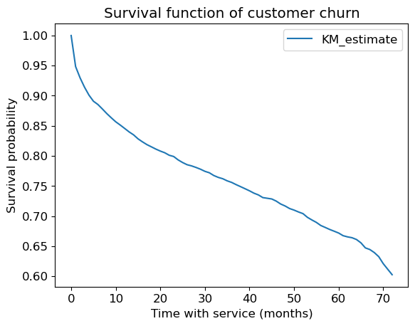
• What is this plot telling us?

• It shows the probability of survival over time.

• For example, after 20 months the probability of survival is ~0.8.

• Over time it’s going down.

What’s the average tenure?

np.mean(train_df_surv["tenure"])

32.6391518364256

What’s the average tenure of the people who churned?

np.mean(train_df_surv.query("Churn == 1.0")["tenure"])

17.854744525547446

What’s the average tenure of the people who did not churn?

np.mean(train_df_surv.query("Churn == 0.0")["tenure"])

37.816717791411044

• Let’s look at the histogram of number of people who have not churned.

• The key point here is that people joined at different times.

plt.figure(figsize=(4, 3))
train_df_surv[train_df_surv['Churn'] == 0]["tenure"].hist(bins=20, grid=False)
plt.xlabel("months");

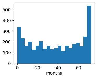
• Since the data was collected at a fixed time and these are the people who hadn’t yet churned, those with larger tenure values here must have joined earlier.

Lifelines can also give us some “error bars”:

kmf.plot_survival_function()
plt.title("Survival function of customer churn")
plt.xlabel("Time with service (months)")
plt.ylabel("Survival probability");

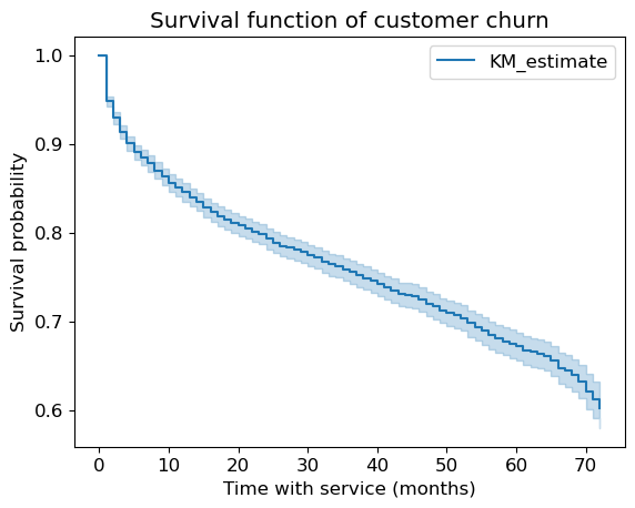
• We already have some actionable information here.

• The curve drops down fast at the beginning suggesting that people tend to leave early on.

• If there would have been a big drop in the curve, it means a bunch of people left at that time (e.g., after a 1-month free trial).

• By the way, the original paper by Kaplan and Meier has been cited over 57000 times!

We can also create the K-M curve for different subgroups:

T = train_df_surv["tenure"]
E = train_df_surv["Churn"]
senior = train_df_surv["SeniorCitizen"] == 1

ax = plt.subplot(111)

kmf.fit(T[senior], event_observed=E[senior], label="Senior Citizens")
kmf.plot_survival_function(ax=ax)

kmf.fit(T[~senior], event_observed=E[~senior], label="Non-Senior Citizens")
kmf.plot_survival_function(ax=ax)

plt.ylim(0, 1)
plt.xlabel("Time with service (months)")
plt.ylabel("Survival probability");

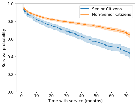
• It looks like senior citizens churn more quickly than others.

• This is quite useful!

Cox proportional hazards model

• We haven’t been incorporating other features in the model so far.

• The Cox proportional hazards model is a commonly used model that allows us to interpret how features influence a censored tenure/duration.

• You can think of it like linear regression for survival analysis: we will get a coefficient for each feature that tells us how it influences survival.

• It makes some strong assumptions (the proportional hazards assumption) that may not be true, but we won’t go into this here.

• The proportional hazard model works multiplicatively, like linear regression with log-transformed targets.

cph = lifelines.CoxPHFitter()
# cph.fit(train_df_surv, duration_col="tenure", event_col="Churn");

• Ok, going to this URL, it seems the easiest solution is to add a penalizer.

  • FYI this is related to switching from LinearRegression to Ridge.

  • Adding drop='first' on our OHE might have helped with this.

  • (For 340 folks: we’re adding regularization; lifelines adds both L1 and L2 regularization, aka elastic net)

cph = lifelines.CoxPHFitter(penalizer=0.1)
cph.fit(train_df_surv, duration_col="tenure", event_col="Churn");

We can look at the coefficients learned by the model and start interpreting them!

cph_params = pd.DataFrame(cph.params_).sort_values(by="coef", ascending=False)
cph_params

	coef
covariate
Contract_Month-to-month	0.812875
OnlineSecurity_No	0.311151
OnlineBackup_No	0.298561
PaymentMethod_Electronic check	0.280801
Partner_No	0.244814
...	...
OnlineBackup_Yes	-0.282600
PaymentMethod_Credit card (automatic)	-0.302801
OnlineSecurity_Yes	-0.330346
Contract_One year	-0.351821
Contract_Two year	-0.776427

43 rows × 1 columns

How to interpret these coefficients In the Cox Proportional Hazards model?

• A positive coefficient indicates that higher values of the feature are associated with higher hazard rates, meaning they are associated with worse survival.

• A negative coefficient indicates that higher values of the feature are associated with lower hazard rates, meaning they are associated with better survival.

• In our example, it looks like Contract_Month-to-month has a positive coefficient

  • If the contract is month-to-month, it leads to more churn worse survival (😔)

• In our example, it looks like Contract_Two year has a negative coefficient

  • If the contract is two-year contract, it leads to less churn better survival (😊)

This makes sense!!!

# cph.baseline_hazard_ # baseline hazard

cph.summary

	coef	exp(coef)	se(coef)	coef lower 95%	coef upper 95%	exp(coef) lower 95%	exp(coef) upper 95%	cmp to	z	p	-log2(p)
covariate
SeniorCitizen	-0.019556	0.980634	0.057254	-0.131773	0.092660	0.876540	1.097088	0.0	-0.341571	0.732674	0.448757
MonthlyCharges	-0.003185	0.996820	0.040129	-0.081837	0.075467	0.921422	1.078387	0.0	-0.079377	0.936733	0.094290
MultipleLines_No	0.162904	1.176924	0.066166	0.033222	0.292587	1.033780	1.339889	0.0	2.462060	0.013814	6.177709
MultipleLines_No phone service	0.014650	1.014758	0.127087	-0.234436	0.263736	0.791017	1.301784	0.0	0.115276	0.908227	0.138876
MultipleLines_Yes	-0.171899	0.842064	0.066810	-0.302844	-0.040954	0.738715	0.959873	0.0	-2.572962	0.010083	6.631899
...	...	...	...	...	...	...	...	...	...	...	...
DeviceProtection_No	0.180214	1.197473	0.067879	0.047174	0.313254	1.048304	1.367868	0.0	2.654935	0.007932	6.978031
DeviceProtection_No internet service	-0.057267	0.944342	0.100970	-0.255165	0.140631	0.774789	1.150999	0.0	-0.567169	0.570599	0.809450
DeviceProtection_Yes	-0.154556	0.856795	0.069302	-0.290385	-0.018727	0.747975	0.981447	0.0	-2.230194	0.025735	5.280148
Dependents_No	0.063772	1.065849	0.075042	-0.083308	0.210852	0.920067	1.234730	0.0	0.849812	0.395429	1.338508
Dependents_Yes	-0.063772	0.938219	0.075042	-0.210852	0.083308	0.809894	1.086877	0.0	-0.849812	0.395429	1.338508

43 rows × 11 columns

Could we have gotten this type of information out of sklearn?

• Yes, let’s try it out!

• But remember that using survival analysis approach is more appropriate for such problems.

y_train.head()

6464     No
5707     No
3442     No
3932    Yes
6124     No
Name: Churn, dtype: object

X_train.drop(columns=["tenure"]).head()

	customerID	gender	SeniorCitizen	Partner	Dependents	PhoneService	MultipleLines	InternetService	OnlineSecurity	OnlineBackup	DeviceProtection	TechSupport	StreamingTV	StreamingMovies	Contract	PaperlessBilling	PaymentMethod	MonthlyCharges	TotalCharges
6464	4726-DLWQN	Male	1	No	No	Yes	Yes	DSL	Yes	Yes	No	No	Yes	No	Month-to-month	Yes	Bank transfer (automatic)	70.35	3454.60
5707	4537-DKTAL	Female	0	No	No	Yes	No	DSL	No	No	No	No	No	No	Month-to-month	No	Electronic check	45.55	84.40
3442	0468-YRPXN	Male	0	No	No	Yes	No	Fiber optic	No	No	Yes	Yes	Yes	Yes	Month-to-month	Yes	Credit card (automatic)	98.80	2807.10
3932	1304-NECVQ	Female	1	No	No	Yes	Yes	Fiber optic	No	No	Yes	No	No	No	Month-to-month	Yes	Electronic check	78.55	149.55
6124	7153-CHRBV	Female	0	Yes	Yes	Yes	No	DSL	Yes	No	Yes	Yes	No	No	One year	Yes	Mailed check	59.30	3274.35

I’m redefining feature types and our preprocessor for our sanity.

numeric_features = ["MonthlyCharges"]
drop_features = ["customerID", "tenure", "TotalCharges"]
passthrough_features = ["SeniorCitizen"]
target_column = ["Churn"]
# the rest are categorical
categorical_features = list(
    set(train_df.columns)
    - set(numeric_features)
    - set(passthrough_features)
    - set(drop_features)
    - set(target_column)
)

preprocessor = make_column_transformer(
    (
        make_pipeline(SimpleImputer(strategy="median"), StandardScaler()),
        numeric_features,
    ),
    (OneHotEncoder(handle_unknown="ignore"), categorical_features),
    ("passthrough", passthrough_features),
    ("drop", drop_features),
)

preprocessor.fit(X_train);

new_columns = (
    numeric_features
    + preprocessor.named_transformers_["onehotencoder"]
    .get_feature_names_out(categorical_features)
    .tolist()
    + passthrough_features
)

lr = make_pipeline(preprocessor, LogisticRegression(max_iter=1000))
lr.fit(X_train, y_train)
lr_coefs = pd.DataFrame(
    data=np.squeeze(lr[1].coef_), index=new_columns, columns=["Coefficient"]
)

lr_coefs.sort_values(by="Coefficient", ascending=False)

	Coefficient
Contract_Month-to-month	1.117063
InternetService_Fiber optic	0.522513
OnlineSecurity_No	0.349206
PaymentMethod_Electronic check	0.311261
OnlineBackup_No	0.253954
...	...
MonthlyCharges	-0.172977
OnlineSecurity_Yes	-0.242936
PaymentMethod_Credit card (automatic)	-0.260652
InternetService_DSL	-0.416242
Contract_Two year	-1.019200

43 rows × 1 columns

• There is some agreement, which is good.

• But our survival model is much more useful.

  • Not to mention more correct.

• One thing we get with lifelines is confidence intervals on the coefficients:

plt.figure(figsize=(10, 12))
cph.plot();

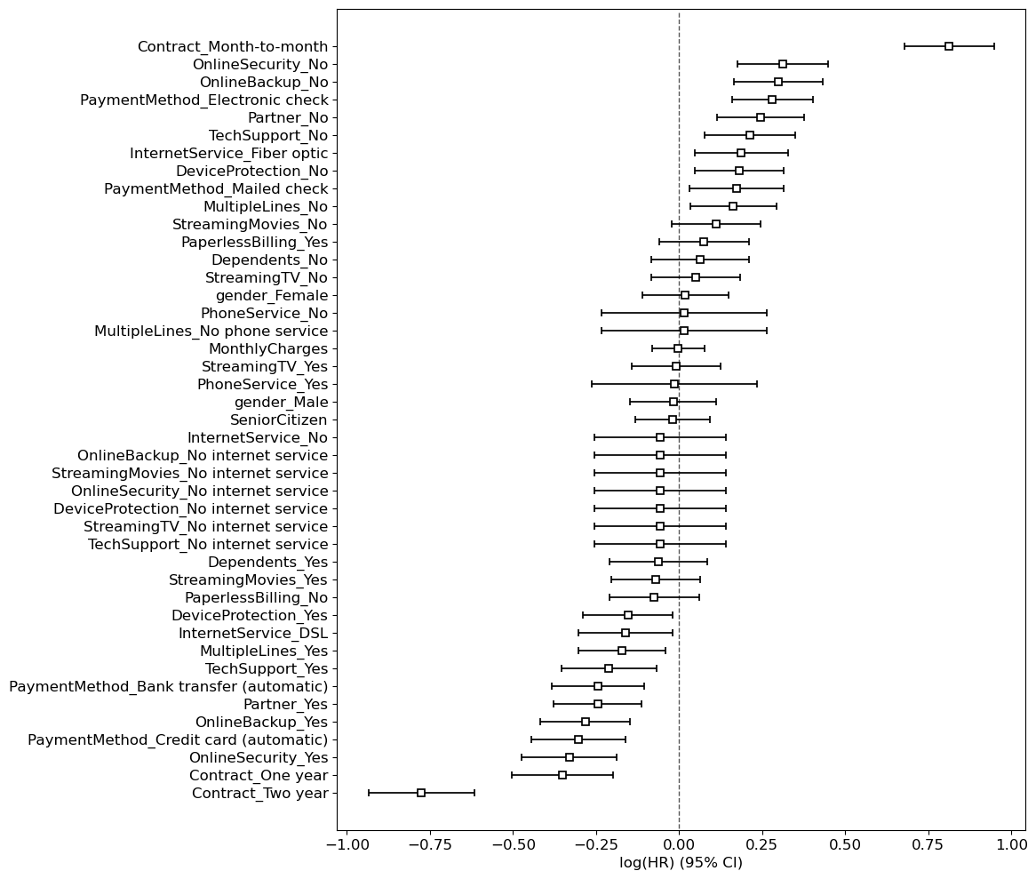
• (We could probably get the same for logistic regression if using statsmodels instead of sklearn.)

• However, in general, I would be careful with all of this.

• Ideally we would have more statistical training when using lifelines - there is a lot that can go wrong.

  • It comes with various diagnostics as well.

• But I think it’s very useful to know about survival analysis and the availability of software to deal with it.

• Oh, and there are lots of other nice plots.

Survival plots

• Let’s look at the survival plots for the people with

  • two-year contract (Contract_Two year = 1) and

  • people without two-year contract (Contract_Two year = 0)

• As expected, the former survive longer.

cph.plot_partial_effects_on_outcome("Contract_Two year", [0, 1]);
plt.xlabel("Time with service (months)")
plt.ylabel("Survival probability");

Now let’s look at the survival plots for the people with different MonthlyCharges.

cph.plot_partial_effects_on_outcome("MonthlyCharges", [10, 100, 1000, 10_000]);
plt.xlabel("Time with service (months)")
plt.ylabel("Survival probability");

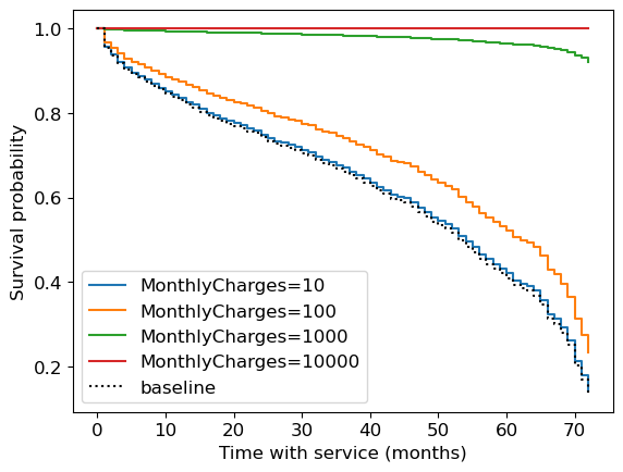
• That’s the thing with linear models, they can’t stop the growth.

• We have a negative coefficient associated with MonthlyCharges

cph_params.loc["MonthlyCharges"]

coef   -0.003185
Name: MonthlyCharges, dtype: float64

If your monthly charges are huge, it takes this to the extreme and thinks you’ll basically never churn.

Prediction

• We can use survival analysis to make predictions as well.

• Here is the expected number of months to churn for the first 5 customers in the test set:

test_X = test_df_surv.drop(columns=["tenure", "Churn"])

How long each non-churned customer is likely to stay according to the model assuming that they just joined right now?

cph.predict_expectation(test_X).head()  # assumes they just joined right now

941     35.206724
1404    69.023086
5515    68.608565
3684    27.565062
7017    67.890933
dtype: float64

Survival curves for first 5 customers in the test set:

cph.predict_survival_function(test_X[:5]).plot()
plt.xlabel("Time with service (months)")
plt.ylabel("Survival probability");

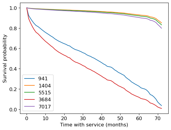
From predict_survival_function documentation:

Predict the survival function for individuals, given their covariates. This assumes that the individual just entered the study (that is, we do not condition on how long they have already lived for.)

So these curves are “starting now”.

• There’s no probability prerequisite for this course, so this is optional material.

• But you can do some interesting stuff here with conditional probabilities.

• “Given that a customer has been here 5 months, what’s the outlook?”

  • It will be different than for a new customer.

  • Thus, we might still want to predict for the non-churned customers in the training set!

  • Not something we really thought about with our traditional supervised learning.

Let’s get the customers who have not churned yet.

train_df_surv_not_churned = train_df_surv[train_df_surv["Churn"] == 0]

We can condition on the person having been around for 20 months.

cph.predict_survival_function(train_df_surv_not_churned[:1], conditional_after=20)

	6464
0.0	1.000000
1.0	0.996788
2.0	0.991966
3.0	0.989443
4.0	0.982570
...	...
68.0	0.429634
69.0	0.429634
70.0	0.429634
71.0	0.429634
72.0	0.429634

73 rows × 1 columns

plt.figure()
cph.predict_survival_function(train_df_surv_not_churned[:1]).plot(ax=plt.gca())
preds = cph.predict_survival_function(
    train_df_surv_not_churned[:1], conditional_after=20
)
plt.plot(preds.index[20:], preds.values[:-20])
plt.xlabel("Time with service (months)")
plt.ylabel("Survival probability")
plt.legend(["Starting now", "Given 20 more months of service"])
plt.ylim([0, 1])
plt.xlim([1, 50]);

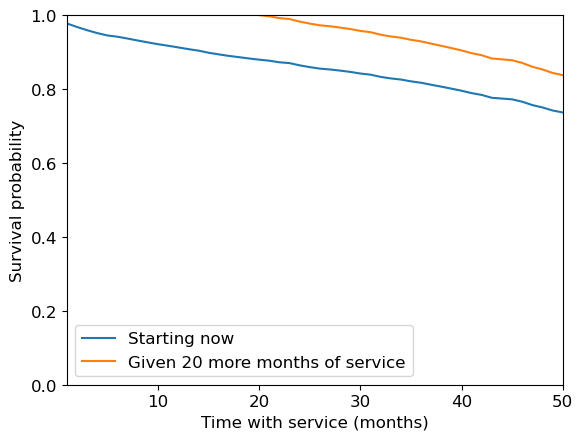
• Look at how the survival function (and expected lifetime) is much longer given that the customer has already lasted 20 months.

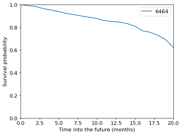
• How long each non-churned customer is likely to stay according to the model assuming that they have been here for the tenure time?

• So, we can set this to their actual tenure so far to get a prediciton of what will happen going forward:

cph.predict_survival_function(
    train_df_surv_not_churned[:1],
    conditional_after=train_df_surv_not_churned[:1]["tenure"],
).plot()
plt.xlabel("Time into the future (months)")
plt.ylabel("Survival probability")
plt.ylim([0, 1])
plt.xlim([0, 20]);

• Another useful application: you could ask what is the customer lifetime value.

  • Basically, how much money do you expect to make off this customer between now and when they churn?

• With regular supervised learning, tenure was a feature and we could only predict whether or not they had churned by then.

(Optional) Evaluation

By default score returns “partial log likelihood”:

cph.score(train_df_surv)

-1.8641864337292489

cph.score(test_df_surv)

-1.7277854625841886

We can look at the “concordance index” which is more interpretable:

cph.concordance_index_

0.8625888648969532

cph.score(train_df_surv, scoring_method="concordance_index")

0.8625888648969532

cph.score(test_df_surv, scoring_method="concordance_index")

0.8546143543902771

From the documentation here:

Another censoring-sensitive measure is the concordance-index, also known as the c-index. This measure evaluates the accuracy of the ranking of predicted time. It is in fact a generalization of AUC, another common loss function, and is interpreted similarly:

• 0.5 is the expected result from random predictions,

• 1.0 is perfect concordance and,

• 0.0 is perfect anti-concordance (multiply predictions with -1 to get 1.0)

Here is an excellent introduction & description of the c-index for new users.

cph.log_likelihood_ratio_test()

null_distribution	chi squared
degrees_freedom	43
test_name	log-likelihood ratio test

	test_statistic	p	-log2(p)
0	2206.68	<0.005	inf

cph.check_assumptions(train_df_surv)

The ``p_value_threshold`` is set at 0.01. Even under the null hypothesis of no violations, some
covariates will be below the threshold by chance. This is compounded when there are many covariates.
Similarly, when there are lots of observations, even minor deviances from the proportional hazard
assumption will be flagged.

With that in mind, it's best to use a combination of statistical tests and visual tests to determine
the most serious violations. Produce visual plots using ``check_assumptions(..., show_plots=True)``
and looking for non-constant lines. See link [A] below for a full example.

null_distribution	chi squared
degrees_of_freedom	1
model	<lifelines.CoxPHFitter: fitted with 5282 total...
test_name	proportional_hazard_test

		test_statistic	p	-log2(p)
Contract_Month-to-month	km	0.07	0.80	0.33
	rank	0.00	0.97	0.04
Contract_One year	km	14.52	<0.005	12.81
	rank	10.11	<0.005	9.41
Contract_Two year	km	8.86	<0.005	8.42
	rank	7.69	0.01	7.49
Dependents_No	km	0.07	0.79	0.34
	rank	0.07	0.79	0.34
Dependents_Yes	km	0.07	0.79	0.34
	rank	0.07	0.79	0.34
DeviceProtection_No	km	0.07	0.79	0.34
	rank	0.08	0.77	0.37
DeviceProtection_No internet service	km	0.25	0.62	0.69
	rank	0.26	0.61	0.72
DeviceProtection_Yes	km	0.70	0.40	1.31
	rank	0.76	0.38	1.38
InternetService_DSL	km	0.32	0.57	0.81
	rank	0.28	0.59	0.75
InternetService_Fiber optic	km	1.02	0.31	1.68
	rank	0.98	0.32	1.64
InternetService_No	km	0.25	0.62	0.69
	rank	0.26	0.61	0.72
MonthlyCharges	km	1.65	0.20	2.33
	rank	1.72	0.19	2.40
MultipleLines_No	km	1.57	0.21	2.25
	rank	1.87	0.17	2.55
MultipleLines_No phone service	km	0.03	0.86	0.21
	rank	0.05	0.83	0.27
MultipleLines_Yes	km	1.92	0.17	2.59
	rank	2.35	0.13	3.00
OnlineBackup_No	km	0.29	0.59	0.76
	rank	0.24	0.63	0.68
OnlineBackup_No internet service	km	0.25	0.62	0.69
	rank	0.26	0.61	0.72
OnlineBackup_Yes	km	1.25	0.26	1.92
	rank	1.17	0.28	1.84
OnlineSecurity_No	km	0.02	0.88	0.19
	rank	0.09	0.77	0.38
OnlineSecurity_No internet service	km	0.25	0.62	0.69
	rank	0.26	0.61	0.72
OnlineSecurity_Yes	km	0.56	0.46	1.13
	rank	0.85	0.36	1.49
PaperlessBilling_No	km	0.03	0.86	0.21
	rank	0.02	0.90	0.16
PaperlessBilling_Yes	km	0.03	0.86	0.21
	rank	0.02	0.90	0.16
Partner_No	km	0.27	0.60	0.73
	rank	0.37	0.54	0.88
Partner_Yes	km	0.27	0.60	0.73
	rank	0.37	0.54	0.88
PaymentMethod_Bank transfer (automatic)	km	0.44	0.51	0.98
	rank	0.51	0.48	1.07
PaymentMethod_Credit card (automatic)	km	1.46	0.23	2.14
	rank	1.70	0.19	2.38
PaymentMethod_Electronic check	km	0.06	0.81	0.30
	rank	0.05	0.82	0.29
PaymentMethod_Mailed check	km	2.36	0.12	3.01
	rank	2.85	0.09	3.45
PhoneService_No	km	0.03	0.86	0.21
	rank	0.05	0.83	0.27
PhoneService_Yes	km	0.03	0.86	0.21
	rank	0.05	0.83	0.27
SeniorCitizen	km	0.00	0.95	0.08
	rank	0.00	0.95	0.08
StreamingMovies_No	km	1.10	0.30	1.76
	rank	1.25	0.26	1.93
StreamingMovies_No internet service	km	0.25	0.62	0.69
	rank	0.26	0.61	0.72
StreamingMovies_Yes	km	2.45	0.12	3.09
	rank	2.73	0.10	3.35
StreamingTV_No	km	1.09	0.30	1.76
	rank	0.90	0.34	1.55
StreamingTV_No internet service	km	0.25	0.62	0.69
	rank	0.26	0.61	0.72
StreamingTV_Yes	km	2.48	0.12	3.12
	rank	2.23	0.14	2.89
TechSupport_No	km	0.49	0.49	1.04
	rank	0.50	0.48	1.07
TechSupport_No internet service	km	0.25	0.62	0.69
	rank	0.26	0.61	0.72
TechSupport_Yes	km	1.92	0.17	2.59
	rank	2.01	0.16	2.68
gender_Female	km	0.22	0.64	0.65
	rank	0.08	0.78	0.35
gender_Male	km	0.22	0.64	0.65
	rank	0.08	0.78	0.35

1. Variable 'Contract_One year' failed the non-proportional test: p-value is 0.0001.

   Advice: with so few unique values (only 2), you can include `strata=['Contract_One year', ...]`
in the call in `.fit`. See documentation in link [E] below.

2. Variable 'Contract_Two year' failed the non-proportional test: p-value is 0.0029.

   Advice: with so few unique values (only 2), you can include `strata=['Contract_Two year', ...]`
in the call in `.fit`. See documentation in link [E] below.

---
[A]  https://lifelines.readthedocs.io/en/latest/jupyter_notebooks/Proportional%20hazard%20assumption.html
[B]  https://lifelines.readthedocs.io/en/latest/jupyter_notebooks/Proportional%20hazard%20assumption.html#Bin-variable-and-stratify-on-it
[C]  https://lifelines.readthedocs.io/en/latest/jupyter_notebooks/Proportional%20hazard%20assumption.html#Introduce-time-varying-covariates
[D]  https://lifelines.readthedocs.io/en/latest/jupyter_notebooks/Proportional%20hazard%20assumption.html#Modify-the-functional-form
[E]  https://lifelines.readthedocs.io/en/latest/jupyter_notebooks/Proportional%20hazard%20assumption.html#Stratification

[]

Other approaches / what did we not cover?

There are many other approaches to modelling in survival analysis:

• Time-varying proportional hazards.

  • What if some of the features change over time, e.g. plan type, number of lines, etc.

• Approaches based on deep learning, e.g. the pysurvival package.

• Random survival forests.

• And more…

Types of censoring

There are also various types and sub-types of censoring we didn’t cover:

• What we did today is called “right censoring”

• Sub-types within right censoring

  • Did everyone join at the same time?

  • Other reasons the data might be censored at random times, e.g. the person died?

• Left censoring

• Interval censoring

Summary

• Censoring and incorrect approaches to handling it

  • Throw away people who haven’t churned

  • Assume everyone churns today

• Predicting tenure vs. churned

• Survival analysis encompasses both of these, and deals with censoring

• And it can make rich and interesting predictions!

• KM model -> doesn’t look at features

• CPH model -> like linear regression, does look at the features

References

Some people working with this same dataset:

• https://medium.com/@zachary.james.angell/applying-survival-analysis-to-customer-churn-40b5a809b05a

• https://towardsdatascience.com/churn-prediction-and-prevention-in-python-2d454e5fd9a5 (Cox)

• https://towardsdatascience.com/survival-analysis-in-python-a-model-for-customer-churn-e737c5242822

• https://towardsdatascience.com/survival-analysis-intuition-implementation-in-python-504fde4fcf8e

lifelines documentation:

• https://lifelines.readthedocs.io/en/latest/Survival%20analysis%20with%20lifelines.html

• https://lifelines.readthedocs.io/en/latest/Survival%20Analysis%20intro.html#introduction-to-survival-analysis