Lecture 3: Class demo

Imports, Announcements, LOs

Imports

# import the libraries
import os
import sys
sys.path.append("../code/.")
from plotting_functions import *
from utils import *

import matplotlib.pyplot as plt
import numpy as np
import pandas as pd

%matplotlib inline

pd.set_option("display.max_colwidth", 200)

Data

Let’s bring back King County housing sale prediction data from the course introduction video. You can download the data from here.

housing_df = pd.read_csv('../data/kc_house_data.csv')
housing_df

	id	date	price	bedrooms	bathrooms	sqft_living	sqft_lot	floors	waterfront	view	...	grade	sqft_above	sqft_basement	yr_built	yr_renovated	zipcode	lat	long	sqft_living15	sqft_lot15
0	7129300520	20141013T000000	221900.0	3	1.00	1180	5650	1.0	0	0	...	7	1180	0	1955	0	98178	47.5112	-122.257	1340	5650
1	6414100192	20141209T000000	538000.0	3	2.25	2570	7242	2.0	0	0	...	7	2170	400	1951	1991	98125	47.7210	-122.319	1690	7639
2	5631500400	20150225T000000	180000.0	2	1.00	770	10000	1.0	0	0	...	6	770	0	1933	0	98028	47.7379	-122.233	2720	8062
3	2487200875	20141209T000000	604000.0	4	3.00	1960	5000	1.0	0	0	...	7	1050	910	1965	0	98136	47.5208	-122.393	1360	5000
4	1954400510	20150218T000000	510000.0	3	2.00	1680	8080	1.0	0	0	...	8	1680	0	1987	0	98074	47.6168	-122.045	1800	7503
...	...	...	...	...	...	...	...	...	...	...	...	...	...	...	...	...	...	...	...	...	...
21608	263000018	20140521T000000	360000.0	3	2.50	1530	1131	3.0	0	0	...	8	1530	0	2009	0	98103	47.6993	-122.346	1530	1509
21609	6600060120	20150223T000000	400000.0	4	2.50	2310	5813	2.0	0	0	...	8	2310	0	2014	0	98146	47.5107	-122.362	1830	7200
21610	1523300141	20140623T000000	402101.0	2	0.75	1020	1350	2.0	0	0	...	7	1020	0	2009	0	98144	47.5944	-122.299	1020	2007
21611	291310100	20150116T000000	400000.0	3	2.50	1600	2388	2.0	0	0	...	8	1600	0	2004	0	98027	47.5345	-122.069	1410	1287
21612	1523300157	20141015T000000	325000.0	2	0.75	1020	1076	2.0	0	0	...	7	1020	0	2008	0	98144	47.5941	-122.299	1020	1357

21613 rows × 21 columns

Exploratory Data Analysis

Is this a classification problem or a regression problem?

# How many data points do we have? 
n = housing_df.shape[0]
n

21613

# What are the columns in the dataset? 
housing_df.columns

Index(['id', 'date', 'price', 'bedrooms', 'bathrooms', 'sqft_living',
       'sqft_lot', 'floors', 'waterfront', 'view', 'condition', 'grade',
       'sqft_above', 'sqft_basement', 'yr_built', 'yr_renovated', 'zipcode',
       'lat', 'long', 'sqft_living15', 'sqft_lot15'],
      dtype='object')

# Do we need to keep all the columns? 
X = housing_df.drop(columns=['id', 'date', 'zipcode', 'price'])

y = housing_df['price']

Let’s explore some features. Let’s try the describe() method

X.describe()

	bedrooms	bathrooms	sqft_living	sqft_lot	floors	waterfront	view	condition	grade	sqft_above	sqft_basement	yr_built	yr_renovated	lat	long	sqft_living15	sqft_lot15
count	21613.000000	21613.000000	21613.000000	2.161300e+04	21613.000000	21613.000000	21613.000000	21613.000000	21613.000000	21613.000000	21613.000000	21613.000000	21613.000000	21613.000000	21613.000000	21613.000000	21613.000000
mean	3.370842	2.114757	2079.899736	1.510697e+04	1.494309	0.007542	0.234303	3.409430	7.656873	1788.390691	291.509045	1971.005136	84.402258	47.560053	-122.213896	1986.552492	12768.455652
std	0.930062	0.770163	918.440897	4.142051e+04	0.539989	0.086517	0.766318	0.650743	1.175459	828.090978	442.575043	29.373411	401.679240	0.138564	0.140828	685.391304	27304.179631
min	0.000000	0.000000	290.000000	5.200000e+02	1.000000	0.000000	0.000000	1.000000	1.000000	290.000000	0.000000	1900.000000	0.000000	47.155900	-122.519000	399.000000	651.000000
25%	3.000000	1.750000	1427.000000	5.040000e+03	1.000000	0.000000	0.000000	3.000000	7.000000	1190.000000	0.000000	1951.000000	0.000000	47.471000	-122.328000	1490.000000	5100.000000
50%	3.000000	2.250000	1910.000000	7.618000e+03	1.500000	0.000000	0.000000	3.000000	7.000000	1560.000000	0.000000	1975.000000	0.000000	47.571800	-122.230000	1840.000000	7620.000000
75%	4.000000	2.500000	2550.000000	1.068800e+04	2.000000	0.000000	0.000000	4.000000	8.000000	2210.000000	560.000000	1997.000000	0.000000	47.678000	-122.125000	2360.000000	10083.000000
max	33.000000	8.000000	13540.000000	1.651359e+06	3.500000	1.000000	4.000000	5.000000	13.000000	9410.000000	4820.000000	2015.000000	2015.000000	47.777600	-121.315000	6210.000000	871200.000000

# What are the value counts of the `waterfront` feature? 
X['waterfront'].value_counts()

waterfront
0    21450
1      163
Name: count, dtype: int64

# What are the value_counts of `yr_renovated` feature? 
X['yr_renovated'].value_counts()

yr_renovated
0       20699
2014       91
2013       37
2003       36
2005       35
        ...  
1951        1
1959        1
1948        1
1954        1
1944        1
Name: count, Length: 70, dtype: int64

Many opportunities to clean the data but we’ll stop here.

Baseline model

# Train a DummyRegressor model 

from sklearn.dummy import DummyRegressor # Import DummyRegressor 

# Create a class object for the sklearn model.
dummy = DummyRegressor()

# fit the dummy regressor
dummy.fit(X, y)

# score the model 
dummy.score(X, y)

0.0

# predict on X using the model
dummy.predict(X)

array([540088.14176653, 540088.14176653, 540088.14176653, ...,
       540088.14176653, 540088.14176653, 540088.14176653])

Decision tree model

# Train a decision tree model 

from sklearn.tree import DecisionTreeRegressor # Import DecisionTreeRegressor 

# Create a class object for the sklearn model.
dt = DecisionTreeRegressor(random_state=123)

# fit the decision tree regressor 
dt.fit(X, y)

# score the model 
dt.score(X, y)

0.9991338290544213

We are getting a perfect accuracy. Should we be happy with this model and deploy it? Why or why not?

What’s the depth of this model?

dt.get_depth()

38

Data splitting

Let’s split the data and

• Train on the train split

• Score on the test split

# Split the data 
from sklearn.model_selection import train_test_split
X_train, X_test, y_train, y_test = train_test_split(X, y, test_size=0.2, random_state=123)

# Instantiate a class object 
dt = DecisionTreeRegressor(random_state=123)

# Train a decision tree on X_train, y_train
dt.fit(X_train, y_train)

# Score on the train set
dt.score(X_train, y_train)

0.9994394006711425

# Score on the test set
dt.score(X_test, y_test)

0.719915905190645

Activity: Discuss the following questions in your group

• Why is there a large gap between train and test scores?

• What would be the effect of increasing or decreasing test_size?

• Why are we setting the random_state? Is it a good idea to try a bunch of values for the random_state and pick the one which gives the best scores?

• Would it be possible to further improve the scores?

Let’s try out different depths.

max_depth= 1 
dt = DecisionTreeRegressor(max_depth=1, random_state=123) 
dt.fit(X_train, y_train)

DecisionTreeRegressor(max_depth=1, random_state=123)

In a Jupyter environment, please rerun this cell to show the HTML representation or trust the notebook.
On GitHub, the HTML representation is unable to render, please try loading this page with nbviewer.org.

# Visualize your decision stump
from sklearn.tree import plot_tree 
plot_tree(dt, feature_names = X.columns.tolist(), impurity=False, filled=True);

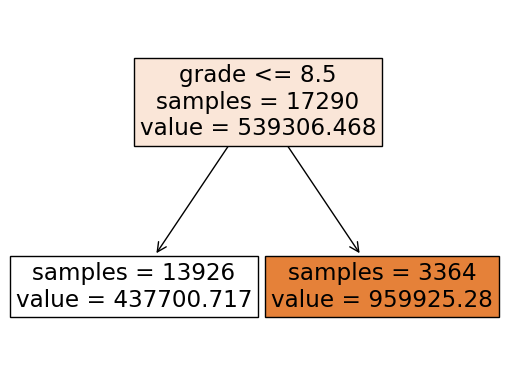
dt.score(X_train, y_train) # Score on the train set

0.3209427041566191

dt.score(X_test, y_test) # Score on the test set

0.31767136668453344

• How do these scores compare to the previous scores?

Let’s try depth 10.

dt = DecisionTreeRegressor(max_depth=10, random_state=123) # max_depth= 10 
dt.fit(X_train, y_train)

DecisionTreeRegressor(max_depth=10, random_state=123)

In a Jupyter environment, please rerun this cell to show the HTML representation or trust the notebook.
On GitHub, the HTML representation is unable to render, please try loading this page with nbviewer.org.

dt.score(X_train, y_train) # Score on the train set

0.9108334653214172

dt.score(X_test, y_test) # Score on the test set

0.7728396574320712

Any improvements? Which depth should we pick?

Single validation set

We are using the test data again and again. How about creating a validation set to pick the right depth and assessing the final model on the test set?

# Create a validation set 
X_tr, X_valid, y_tr, y_valid = train_test_split(X_train, y_train, test_size=0.2, random_state=123)

tr_scores = []
valid_scores = []
depths = np.arange(1, 35, 2)
for depth in depths:    
    # Create and fit a decision tree model for the given depth  
    dt = DecisionTreeRegressor(max_depth=depth, random_state=123)
    dt.fit(X_tr, y_tr)
    
    # Calculate and append r2 scores on the training and validation sets
    tr_scores.append(dt.score(X_tr, y_tr))
    valid_scores.append(dt.score(X_valid, y_valid))
    
results_single_valid_df = pd.DataFrame({"train_score": tr_scores, 
                           "valid_score": valid_scores},index = depths)
results_single_valid_df

	train_score	valid_score
1	0.319559	0.326616
3	0.603739	0.555180
5	0.754938	0.677567
7	0.833913	0.737285
9	0.890456	0.763480
11	0.931896	0.790521
13	0.963024	0.769030
15	0.981643	0.752728
17	0.991810	0.735637
19	0.996424	0.745925
21	0.998370	0.734048
23	0.999213	0.741060
25	0.999480	0.722873
27	0.999544	0.723951
29	0.999558	0.734986
31	0.999562	0.724068
33	0.999567	0.724410

results_single_valid_df[['train_score', 'valid_score']].plot(ylabel='r2 scores');

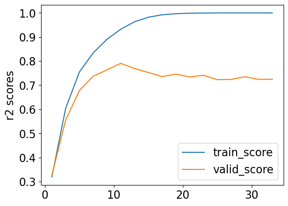
What depth gives the “best” validation score?

best_depth = results_single_valid_df.index.values[np.argmax(results_single_valid_df['valid_score'])]

best_depth

11

Let’s assess the best model on the test set.

test_model = DecisionTreeRegressor(max_depth=best_depth, random_state=123)
test_model.fit(X_train, y_train)
test_model.score(X_test, y_test)

0.7784948928666875

• How do the test scores compare to the validation scores?

• Can we have a more robust estimate of the test score?

Cross-validation

depths = np.arange(1, 35, 2)

cv_train_scores = []
cv_valid_scores = []
for depth in depths: 
    # Create and fit a decision tree model for the given depth   
    dt = DecisionTreeRegressor(max_depth = depth, random_state=123)

    # Carry out cross-validation
    scores = cross_validate(dt, X_train, y_train, return_train_score=True)
    cv_train_scores.append(scores['train_score'].mean())
    cv_valid_scores.append(scores['test_score'].mean())

results_df = pd.DataFrame({"train_score": cv_train_scores, 
                           "valid_score": cv_valid_scores
                           },
                           index=depths
                            )
results_df

	train_score	valid_score
1	0.321050	0.322465
3	0.603243	0.559284
5	0.752169	0.688484
7	0.835876	0.758259
9	0.894960	0.768184
11	0.938201	0.772185
13	0.966812	0.760966
15	0.983340	0.754620
17	0.992220	0.730025
19	0.996487	0.722803
21	0.998440	0.726659
23	0.999178	0.730704
25	0.999438	0.711356
27	0.999518	0.721917
29	0.999539	0.729374
31	0.999545	0.740319
33	0.999546	0.706489

results_df[['train_score', 'valid_score']].plot(ylabel='r2 score', title='Housing price prediction depth vs. r2 score');

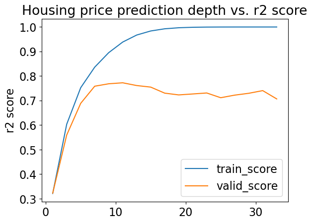
What’s the “best” depth with cross-validation?

best_depth = results_df.index.values[np.argmax(results_df['valid_score'])]
best_depth

11

Discuss the following questions in your group

1. For which depth(s) we are underfitting? How about overfitting?

2. Above we are picking the depth which gives us the best cross-validation score. Is it always a good idea to pick such a depth? What if you have a much simpler model (smaller max_depth), which gives us almost the same CV scores?

3. If we care about the test scores in the end, why don’t we use it in training?

4. Do you trust our hyperparameter optimization? In other words, do you believe that we have found the best possible depth?

Assessing on the test set

dt_final = DecisionTreeRegressor(max_depth=best_depth, random_state=123)
dt_final.fit(X_train, y_train)
dt_final.score(X_train, y_train)

0.9308647034083802

dt_final.score(X_test, y_test)

0.7784948928666875

How do these scores compare to the scores when we used a single validation set?

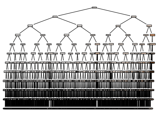
Learned model

#What's the depth of the model? 
dt_final.get_depth()

11

plot_tree(dt_final, feature_names = X_train.columns.tolist(), impurity=False, filled=True);

# Which features are the most important ones?
dt_final.feature_importances_

array([0.00080741, 0.00327551, 0.25123925, 0.01808825, 0.00079645,
       0.03213916, 0.01190633, 0.00106308, 0.36400802, 0.02313684,
       0.00295235, 0.01209545, 0.00064647, 0.17216105, 0.06835056,
       0.02416048, 0.01317334])

Let’s examine feature importances.

df = pd.DataFrame( 
    data = {
        "features": dt_final.feature_names_in_,
        "feature_importances": dt_final.feature_importances_
    }
)
df.sort_values("feature_importances", ascending=False)

	features	feature_importances
8	grade	0.364008
2	sqft_living	0.251239
13	lat	0.172161
14	long	0.068351
5	waterfront	0.032139
15	sqft_living15	0.024160
9	sqft_above	0.023137
3	sqft_lot	0.018088
16	sqft_lot15	0.013173
11	yr_built	0.012095
6	view	0.011906
1	bathrooms	0.003276
10	sqft_basement	0.002952
7	condition	0.001063
0	bedrooms	0.000807
4	floors	0.000796
12	yr_renovated	0.000646