Lectures 7: Class demo#
import os
import sys

sys.path.append("../code/.")

import IPython
import matplotlib.pyplot as plt
import mglearn
import numpy as np
import pandas as pd
from plotting_functions import *
from sklearn.dummy import DummyClassifier
from sklearn.feature_extraction.text import CountVectorizer
from sklearn.model_selection import cross_val_score, cross_validate, train_test_split
from sklearn.pipeline import make_pipeline
from sklearn.linear_model import LogisticRegression
from utils import *

%matplotlib inline
pd.set_option("display.max_colwidth", 200)
Demo: Model interpretation of linear classifiers#
One of the primary advantages of linear classifiers is their ability to interpret models.
For instance, by analyzing the sign and magnitude of the learned coefficients, we can address questions regarding which features are influencing the prediction and in which direction.
We’ll demonstrate this by training
LogisticRegressionon the famous IMDB movie review dataset. The dataset is a bit large for demonstration purposes. So I am going to put a big portion of it in the test split to speed things up.
imdb_df = pd.read_csv("../data/imdb_master.csv", encoding="ISO-8859-1")
imdb_df = imdb_df[imdb_df["label"].str.startswith(("pos", "neg"))]
imdb_df.drop(["Unnamed: 0", "type", "file"], axis=1, inplace=True)
imdb_df.head()
| review | label | |
|---|---|---|
| 0 | Once again Mr. Costner has dragged out a movie for far longer than necessary. Aside from the terrific sea rescue sequences, of which there are very few I just did not care about any of the charact... | neg |
| 1 | This is an example of why the majority of action films are the same. Generic and boring, there's really nothing worth watching here. A complete waste of the then barely-tapped talents of Ice-T and... | neg |
| 2 | First of all I hate those moronic rappers, who could'nt act if they had a gun pressed against their foreheads. All they do is curse and shoot each other and acting like cliché'e version of gangst... | neg |
| 3 | Not even the Beatles could write songs everyone liked, and although Walter Hill is no mop-top he's second to none when it comes to thought provoking action movies. The nineties came and social pla... | neg |
| 4 | Brass pictures (movies is not a fitting word for them) really are somewhat brassy. Their alluring visual qualities are reminiscent of expensive high class TV commercials. But unfortunately Brass p... | neg |
Let’s clean up the data a bit.
import re

def replace_tags(doc):
    doc = doc.replace("<br />", " ")
    doc = re.sub("https://\S*", "", doc)
    return doc
imdb_df["review_pp"] = imdb_df["review"].apply(replace_tags)
Are we breaking the Golden rule here?
Let’s split the data and create bag of words representation.
# imdb_df
train_df, test_df = train_test_split(imdb_df, test_size=0.9, random_state=123)
X_train, y_train = train_df["review_pp"], train_df["label"]
X_test, y_test = test_df["review_pp"], test_df["label"]
train_df.shape
(5000, 3)
X_train
47278    Best animated movie ever made. This film explores not only the vast world of modern animation with absolutely boggling effects, but the branches of the human mind, soul, and philosophy. The story ...
19664    This film does for Infantry what Das Boot did for Submariners. If you appreciated Das Boot then that is all you really need to know.  This is a well done piece of cinema. On a par with Das Boot. B...
22648    New Yorkers contemporaneous with this film will recall how reflective of its time it is and how well cast and crew captured America, New York City of that era.  Norman Wexler's script delineates t...
33662    Well, you might not actually SEE any women in love in this movie, but you'll certainly hear women TALKING about love, and men talking about love, and women talking about men, and men talking about...
31230    Well I just gave away 95 minutes and 47 seconds that I'll never get back on this piece of trash. I heard someone online describe this movie's villains as "subhuman cannibals", and I thought it was...
                                                                                                          ...
7763     I actually went into this film with some expectations, not because I thought the film sounded particularly good, but because I'm a fan of Italian exploitation flicks and with a cast that sees Fran...
15377    SPOILER ALERT! Don't read on unless you're prepared for some spoilers.  I think this film had a lot beneath its shell. Besides the apparent connections with "Oldboy" (and Park-wook's other films),...
17730    A stunning film which brought into the open so much about disability that generally makes people afraid. It showed how minds can be captured by less than willing bodies and how difficult it must b...
28030    this film has its good points: hot chicks people die  the problem... the hot Chicks barley get nude and you don't get to see many of the people dieing, mostly just lots of fast movements and screa...
15725    Run, don't walk, to rent this movie. It is re-released on an excellent DVD version. It is primo acting/directing/cinematography in the world of suspense/film noir. Tribute this to the blacklisted ...
Name: review_pp, Length: 5000, dtype: object
Is there any missing data?
train_df.isna().sum()
review       0
label        0
review_pp    0
dtype: int64
There is no missing data. We don’t need imputation.
# Let's try CountVectorizer
vec = CountVectorizer(max_features=10_000, stop_words="english")
bow = vec.fit_transform(X_train)
bow
<5000x10000 sparse matrix of type '<class 'numpy.int64'>'
	with 383702 stored elements in Compressed Sparse Row format>
Examining the vocabulary#
The vocabulary (mapping from feature indices to actual words) can be obtained using
get_feature_names()on theCountVectorizerobject.
vocab = vec.get_feature_names_out()
vocab[0:10] # first few words
array(['00', '000', '01', '10', '100', '1000', '101', '11', '12', '13'],
      dtype=object)
vocab[2000:2010] # some middle words
array(['conrad', 'cons', 'conscience', 'conscious', 'consciously',
       'consciousness', 'consequence', 'consequences', 'conservative',
       'conservatory'], dtype=object)
vocab[::500] # words with a step of 500
array(['00', 'announcement', 'bird', 'cell', 'conrad', 'depth', 'elite',
       'finnish', 'grimy', 'illusions', 'kerr', 'maltin', 'narrates',
       'patients', 'publicity', 'reynolds', 'sfx', 'starting', 'thats',
       'vance'], dtype=object)
Model building on the dataset#
First let’s try DummyClassifier on the dataset.
dummy = DummyClassifier()
cross_val_score(dummy, X_train, y_train).mean()
0.505
We have a balanced dataset. So the DummyClassifier score is around 0.5.
Now let’s try logistic regression.
# Create a pipeline with CountVectorizer and LogisticRegression
pipe_lr = make_pipeline(CountVectorizer(max_features=10_000, stop_words="english"),
                        LogisticRegression(max_iter=1000)
                       )
scores = cross_validate(pipe_lr, X_train, y_train, return_train_score=True)
pd.DataFrame(scores)
| fit_time | score_time | test_score | train_score | |
|---|---|---|---|---|
| 0 | 0.610184 | 0.091054 | 0.847 | 1.0 |
| 1 | 0.492177 | 0.090021 | 0.832 | 1.0 |
| 2 | 0.497612 | 0.102035 | 0.842 | 1.0 |
| 3 | 0.486308 | 0.086881 | 0.853 | 1.0 |
| 4 | 0.490192 | 0.089057 | 0.839 | 1.0 |
Seems like we are overfitting. Let’s optimize the hyperparameter C.
scores_dict = {
    "C": 10.0 ** np.arange(-3, 3, 1),
    "mean_train_scores": list(),
    "mean_cv_scores": list(),
}
for C in scores_dict["C"]:
    pipe_lr = make_pipeline(CountVectorizer(max_features=10_000, stop_words="english"),
                        LogisticRegression(max_iter=1000, C=C)
                       )
    scores = cross_validate(pipe_lr, X_train, y_train, return_train_score=True)
    scores_dict["mean_train_scores"].append(scores["train_score"].mean())
    scores_dict["mean_cv_scores"].append(scores["test_score"].mean())

results_df = pd.DataFrame(scores_dict)
results_df
| C | mean_train_scores | mean_cv_scores | |
|---|---|---|---|
| 0 | 0.001 | 0.83470 | 0.7964 |
| 1 | 0.010 | 0.92265 | 0.8456 |
| 2 | 0.100 | 0.98585 | 0.8520 |
| 3 | 1.000 | 1.00000 | 0.8426 |
| 4 | 10.000 | 1.00000 | 0.8376 |
| 5 | 100.000 | 1.00000 | 0.8350 |
optimized_C = results_df["C"].iloc[np.argmax(results_df["mean_cv_scores"])]
print(
    "The maximum validation score is %0.3f at C = %0.2f "
    % (
        np.max(results_df["mean_cv_scores"]),
        optimized_C,
    )
)
The maximum validation score is 0.852 at C = 0.10
Let’s train a model on the full training set with the optimized hyperparameter values.
pipe_lr = make_pipeline(CountVectorizer(max_features=10000, stop_words="english"),
                        LogisticRegression(max_iter=1000, C = 0.10)
                       )
pipe_lr.fit(X_train, y_train)
Pipeline(steps=[('countvectorizer',
                 CountVectorizer(max_features=10000, stop_words='english')),
                ('logisticregression',
                 LogisticRegression(C=0.1, max_iter=1000))])
In a Jupyter environment, please rerun this cell to show the HTML representation or trust the notebook. On GitHub, the HTML representation is unable to render, please try loading this page with nbviewer.org.
Pipeline(steps=[('countvectorizer',
                 CountVectorizer(max_features=10000, stop_words='english')),
                ('logisticregression',
LogisticRegression(C=0.1, max_iter=1000))])CountVectorizer(max_features=10000, stop_words='english')
LogisticRegression(C=0.1, max_iter=1000)
Examining learned coefficients#
The learned coefficients are exposed by the
coef_attribute of LogisticRegression object.
feature_names = np.array(pipe_lr.named_steps["countvectorizer"].get_feature_names_out())
coeffs = pipe_lr.named_steps["logisticregression"].coef_.flatten()
# feature_names
word_coeff_df = pd.DataFrame(coeffs, index=feature_names, columns=["Coefficient"])
word_coeff_df
| Coefficient | |
|---|---|
| 00 | -0.074949 |
| 000 | -0.083893 |
| 01 | -0.034402 |
| 10 | 0.056493 |
| 100 | 0.041633 |
| ... | ... |
| zoom | -0.013299 |
| zooms | -0.022139 |
| zorak | 0.021878 |
| zorro | 0.130075 |
| â½ | 0.012649 |
10000 rows × 1 columns
Let’s sort the coefficients in descending order.
Interpretation
if \(w_j > 0\) then increasing \(x_{ij}\) moves us toward predicting \(+1\).
if \(w_j < 0\) then increasing \(x_{ij}\) moves us toward predicting \(-1\).
word_coeff_df.sort_values(by="Coefficient", ascending=False)
| Coefficient | |
|---|---|
| excellent | 0.903484 |
| great | 0.659922 |
| amazing | 0.653301 |
| wonderful | 0.651763 |
| favorite | 0.607887 |
| ... | ... |
| terrible | -0.621695 |
| boring | -0.701030 |
| bad | -0.736608 |
| waste | -0.799353 |
| worst | -0.986970 |
10000 rows × 1 columns
The coefficients make sense!
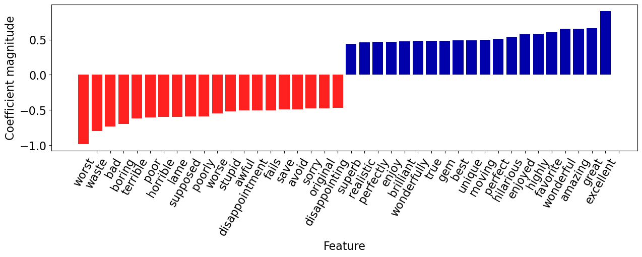
Let’s visualize the top 20 features.
mglearn.tools.visualize_coefficients(coeffs, feature_names, n_top_features=20)
Let’s explore prediction of the following new review.
fake_review = "It got a bit boring at times but the direction was excellent and the acting was flawless. Overall I enjoyed the movie and I highly recommend it!"
feat_vec = pipe_lr.named_steps["countvectorizer"].transform([fake_review])
feat_vec
<1x10000 sparse matrix of type '<class 'numpy.int64'>'
	with 13 stored elements in Compressed Sparse Row format>
Let’s get prediction probability scores of the fake review.
pipe_lr.predict_proba([fake_review])
array([[0.16423497, 0.83576503]])
pipe_lr.classes_
array(['neg', 'pos'], dtype=object)
The model is 83.5% confident that it’s a positive review.
pipe_lr.predict([fake_review])[0]
'pos'
We can find which of the vocabulary words are present in this review:
feat_vec.toarray().ravel().astype(bool)
array([False, False, False, ..., False, False, False])
words_in_ex = feat_vec.toarray().ravel().astype(bool)
words_in_ex
array([False, False, False, ..., False, False, False])
How many of the words are in this review?
np.sum(words_in_ex)
13
np.array(feature_names)[words_in_ex]
array(['acting', 'bit', 'boring', 'direction', 'enjoyed', 'excellent',
       'flawless', 'got', 'highly', 'movie', 'overall', 'recommend',
       'times'], dtype=object)
ex_df = pd.DataFrame(
    data=coeffs[words_in_ex],
    index=np.array(feature_names)[words_in_ex],
    columns=["Coefficient"],
)
ex_df
| Coefficient | |
|---|---|
| acting | -0.126498 |
| bit | 0.390053 |
| boring | -0.701030 |
| direction | -0.268316 |
| enjoyed | 0.578879 |
| excellent | 0.903484 |
| flawless | 0.113743 |
| got | -0.122759 |
| highly | 0.582012 |
| movie | -0.037942 |
| overall | 0.136288 |
| recommend | 0.054205 |
| times | 0.133895 |
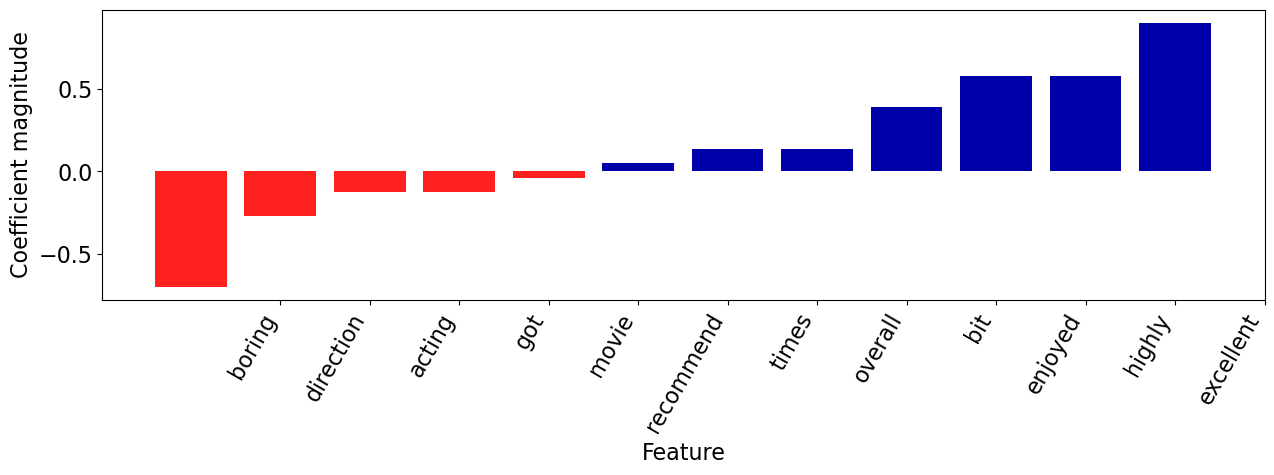
Let’s visualize how the words with positive and negative coefficients are driving the prediction.
mglearn.tools.visualize_coefficients(
    coeffs[words_in_ex], np.array(feature_names)[words_in_ex], n_top_features=6
)
def plot_coeff_example(feat_vect, coeffs, feature_names):
    words_in_ex = feat_vec.toarray().ravel().astype(bool)

    ex_df = pd.DataFrame(
        data=coeffs[words_in_ex],
        index=np.array(feature_names)[words_in_ex],
        columns=["Coefficient"],
    )
    return ex_df
Most positive review#
Remember that you can look at the probabilities (confidence) of the classifier’s prediction using the
model.predict_probamethod.Can we find the reviews where our classifier is most confident or least confident?
pos_probs = pipe_lr.predict_proba(X_train)[
    :, 1
]  # only get probabilities associated with pos class
pos_probs
array([0.95205899, 0.83301769, 0.9093526 , ..., 0.89247531, 0.05736279,
       0.79360853])
Let’s get the index of the example where the classifier is most confident (highest predict_proba score for positive).
most_positive = np.argmax(pos_probs)
X_train.iloc[most_positive]
'Moving beyond words is this heart breaking story of a divorce which results in a tragic custody battle over a seven year old boy. One of "Kramer v. Kramer\'s" great strengths is its screenwriter director Robert Benton, who has marvellously adapted Avery Corman\'s novel to the big screen. He keeps things beautifully simple and most realistic, while delivering all the drama straight from the heart. His talent for telling emotional tales like this was to prove itself again with "Places in the Heart", where he showed, as in "Kramer v. Kramer", that he has a natural ability for working with children. The picture\'s other strong point is the splendid acting which deservedly received four of the film\'s nine Academy Award nominations, two of them walking away winners. One of those was Dustin Hoffman (Best Actor), who is superb as frustrated business man Ted Kramer, a man who has forgotten that his wife is a person. As said wife Joanne, Meryl Streep claimed the supporting actress Oscar for a strong, sensitive portrayal of a woman who had lost herself in eight years of marriage. Also nominated was Jane Alexander for her fantastic turn as the Kramer\'s good friend Margaret. Final word in the acting stakes must go to young Justin Henry, whose incredibly moving performance will find you choking back tears again and again, and a thoroughly deserved Oscar nomination came his way. Brilliant also is Nestor Almendros\' cinematography and Jerry Greenberg\'s timely editing, while musically Henry Purcell\'s classical piece is used to effect. Truly this is a touching story of how a father and son come to depend on each other when their wife and mother leaves. They grow together, come to know each other and form an entirely new and wonderful relationship. Ted finds himself with new responsibilities and a new outlook on life, and slowly comes to realise why Joanne had to go. Certainly if nothing else, "Kramer v. Kramer" demonstrates that nobody wins when it comes to a custody battle over a young child, especially not the child himself. Saturday, June 10, 1995 - T.V. Strong drama from Avery Corman\'s novel about the heartache of a custody battle between estranged parents who both feel they have the child\'s best interests at heart. Aside from a superb screenplay and amazingly controlled direction, both from Robert Benton, it\'s the superlative cast that make this picture such a winner. Hoffman is brilliant as Ted Kramer, the man torn between his toppling career and the son whom he desperately wants to keep. Excellent too is Streep as the woman lost in eight years of marriage who had to get out before she faded to nothing as a person. In support of these two is a very strong Jane Alexander as mutual friend Margaret, an outstanding Justin Henry as the boy caught in the middle, and a top cast of extras. This highly emotional, heart rending drama more than deserved it\'s 1979 Academy Awards for best film, best actor (Hoffman) and best supporting actress (Streep). Wednesday, February 28, 1996 - T.V.'
print("True target: %s\n" % (y_train.iloc[most_positive]))
print("Predicted target: %s\n" % (pipe_lr.predict(X_train.iloc[[most_positive]])[0]))
print("Prediction probability: %0.4f" % (pos_probs[most_positive]))
True target: pos

Predicted target: pos

Prediction probability: 1.0000
Let’s examine the features associated with the review.
feat_vec = pipe_lr.named_steps["countvectorizer"].transform(
    X_train.iloc[[most_positive]]
)
words_in_ex = feat_vec.toarray().ravel().astype(bool)
mglearn.tools.visualize_coefficients(
    coeffs[words_in_ex], np.array(feature_names)[words_in_ex], n_top_features=20
)
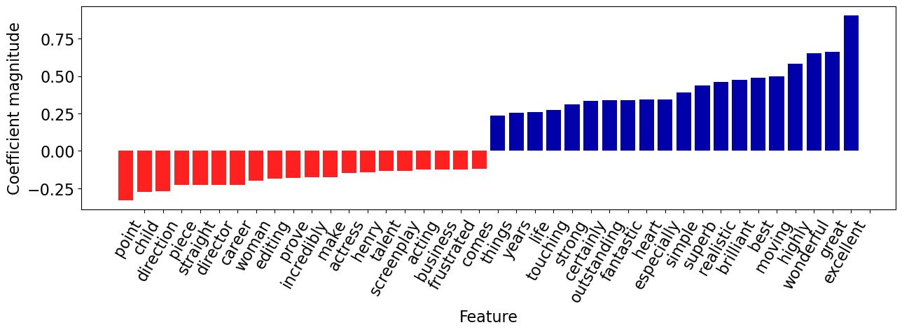
The review has both positive and negative words but the words with positive coefficients win in this case!
Most negative review#
neg_probs = pipe_lr.predict_proba(X_train)[
    :, 0
]  # only get probabilities associated with pos class
neg_probs
array([0.04794101, 0.16698231, 0.0906474 , ..., 0.10752469, 0.94263721,
       0.20639147])
most_negative = np.argmax(neg_probs)
print("Review: %s\n" % (X_train.iloc[[most_negative]]))
print("True target: %s\n" % (y_train.iloc[most_negative]))
print("Predicted target: %s\n" % (pipe_lr.predict(X_train.iloc[[most_negative]])[0]))
print("Prediction probability: %0.4f" % (pos_probs[most_negative]))
Review: 36555    I made the big mistake of actually watching this whole movie a few nights ago. God I'm still trying to recover. This movie does not even deserve a 1.4 average. IMDb needs to have 0 vote ratings po...
Name: review_pp, dtype: object

True target: neg

Predicted target: neg

Prediction probability: 0.0000
feat_vec = pipe_lr.named_steps["countvectorizer"].transform(
    X_train.iloc[[most_negative]]
)
words_in_ex = feat_vec.toarray().ravel().astype(bool)
mglearn.tools.visualize_coefficients(
    coeffs[words_in_ex], np.array(feature_names)[words_in_ex], n_top_features=20
)
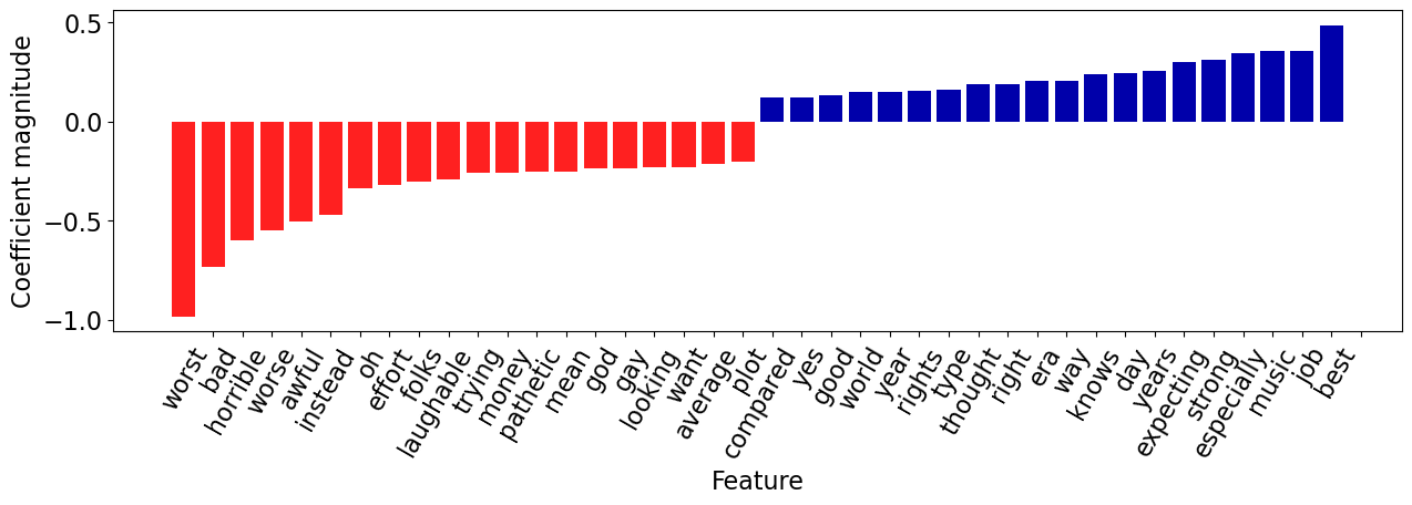
The review has both positive and negative words but the words with negative coefficients win in this case!
❓❓ Questions for you#
Question for you to ponder on#
Is it possible to identify most important features using \(k\)-NNs? What about decision trees?