Lecture 6: sklearn ColumnTransformer and Text Features

Lecture 6: `sklearn` `ColumnTransformer` and Text Features#

UBC 2023-24

Instructor: Varada Kolhatkar and Andrew Roth

Imports, Announcements, and LO#

Imports#

import os
import sys

import matplotlib.pyplot as plt
import numpy as np
import pandas as pd
from IPython.display import HTML

sys.path.append("code/.")
from plotting_functions import *
from utils import *

pd.set_option("display.max_colwidth", 200)

from sklearn.compose import ColumnTransformer, make_column_transformer
from sklearn.dummy import DummyClassifier, DummyRegressor
from sklearn.impute import SimpleImputer
from sklearn.model_selection import cross_val_score, cross_validate, train_test_split
from sklearn.neighbors import KNeighborsClassifier
from sklearn.pipeline import Pipeline, make_pipeline
from sklearn.preprocessing import OneHotEncoder, OrdinalEncoder, StandardScaler
from sklearn.svm import SVC
from sklearn.tree import DecisionTreeClassifier

Learning outcomes#

From this lecture, you will be able to

use ColumnTransformer to build all our transformations together into one object and use it with sklearn pipelines;
define ColumnTransformer where transformers contain more than one steps;
explain handle_unknown="ignore" hyperparameter of scikit-learn’s OneHotEncoder;
explain drop="if_binary" argument of OneHotEncoder;
identify when it’s appropriate to apply ordinal encoding vs one-hot encoding;
explain strategies to deal with categorical variables with too many categories;
explain why text data needs a different treatment than categorical variables;
use scikit-learn’s CountVectorizer to encode text data;
explain different hyperparameters of CountVectorizer.
incorporate text features in a machine learning pipeline

sklearn’s `ColumnTransformer`#

In most applications, some features are categorical, some are continuous, some are binary, and some are ordinal.
When we want to develop supervised machine learning pipelines on real-world datasets, very often we want to apply different transformation on different columns.
Enter sklearn’s ColumnTransformer!!

Let’s look at a toy example:

df = pd.read_csv("data/quiz2-grade-toy-col-transformer.csv")
df

	enjoy_course	ml_experience	major	class_attendance	university_years	lab1	lab2	lab3	lab4	quiz1	quiz2
0	yes	1	Computer Science	Excellent	3	92	93.0	84	91	92	A+
1	yes	1	Mechanical Engineering	Average	2	94	90.0	80	83	91	not A+
2	yes	0	Mathematics	Poor	3	78	85.0	83	80	80	not A+
3	no	0	Mathematics	Excellent	3	91	NaN	92	91	89	A+
4	yes	0	Psychology	Good	4	77	83.0	90	92	85	A+
5	no	1	Economics	Good	5	70	73.0	68	74	71	not A+
6	yes	1	Computer Science	Excellent	4	80	88.0	89	88	91	A+
7	no	0	Mechanical Engineering	Poor	3	95	93.0	69	79	75	not A+
8	no	0	Linguistics	Average	2	97	90.0	94	82	80	not A+
9	yes	1	Mathematics	Average	4	95	82.0	94	94	85	not A+
10	yes	0	Psychology	Good	3	98	86.0	95	95	78	A+
11	yes	1	Physics	Average	1	95	88.0	93	92	85	A+
12	yes	1	Physics	Excellent	2	98	96.0	96	99	100	A+
13	yes	0	Mechanical Engineering	Excellent	4	95	94.0	96	95	100	A+
14	no	0	Mathematics	Poor	3	95	90.0	93	95	70	not A+
15	no	1	Computer Science	Good	3	92	85.0	67	94	92	not A+
16	yes	0	Computer Science	Average	5	75	91.0	93	86	85	A+
17	yes	1	Economics	Average	3	86	89.0	65	86	87	not A+
18	no	1	Biology	Good	2	91	NaN	90	88	82	not A+
19	no	0	Psychology	Poor	2	77	94.0	87	81	89	not A+
20	yes	1	Linguistics	Excellent	4	96	92.0	92	96	87	A+

df.info()

<class 'pandas.core.frame.DataFrame'>
RangeIndex: 21 entries, 0 to 20
Data columns (total 11 columns):
 #   Column            Non-Null Count  Dtype  
---  ------            --------------  -----  
 0   enjoy_course      21 non-null     object 
 1   ml_experience     21 non-null     int64  
 2   major             21 non-null     object 
 3   class_attendance  21 non-null     object 
 4   university_years  21 non-null     int64  
 5   lab1              21 non-null     int64  
 6   lab2              19 non-null     float64
 7   lab3              21 non-null     int64  
 8   lab4              21 non-null     int64  
 9   quiz1             21 non-null     int64  
 10  quiz2             21 non-null     object 
dtypes: float64(1), int64(6), object(4)
memory usage: 1.9+ KB

Transformations on the toy data#

df.head()

	enjoy_course	ml_experience	major	class_attendance	university_years	lab1	lab2	lab3	lab4	quiz1	quiz2
0	yes	1	Computer Science	Excellent	3	92	93.0	84	91	92	A+
1	yes	1	Mechanical Engineering	Average	2	94	90.0	80	83	91	not A+
2	yes	0	Mathematics	Poor	3	78	85.0	83	80	80	not A+
3	no	0	Mathematics	Excellent	3	91	NaN	92	91	89	A+
4	yes	0	Psychology	Good	4	77	83.0	90	92	85	A+

Scaling on numeric features
One-hot encoding on the categorical feature major and binary feature enjoy_class
Ordinal encoding on the ordinal feature class_attendance
Imputation on the lab2 feature
None on the ml_experience feature

`ColumnTransformer` example#

Data#

X = df.drop(columns=["quiz2"])
y = df["quiz2"]
X.columns

Index(['enjoy_course', 'ml_experience', 'major', 'class_attendance',
       'university_years', 'lab1', 'lab2', 'lab3', 'lab4', 'quiz1'],
      dtype='object')

Identify the transformations we want to apply#

X.head()

	enjoy_course	ml_experience	major	class_attendance	university_years	lab1	lab2	lab3	lab4	quiz1
0	yes	1	Computer Science	Excellent	3	92	93.0	84	91	92
1	yes	1	Mechanical Engineering	Average	2	94	90.0	80	83	91
2	yes	0	Mathematics	Poor	3	78	85.0	83	80	80
3	no	0	Mathematics	Excellent	3	91	NaN	92	91	89
4	yes	0	Psychology	Good	4	77	83.0	90	92	85

numeric_feats = ["university_years", "lab1", "lab3", "lab4", "quiz1"]  # apply scaling
categorical_feats = ["major"]  # apply one-hot encoding
passthrough_feats = ["ml_experience"]  # do not apply any transformation
drop_feats = [
    "lab2",
    "class_attendance",
    "enjoy_course",
]  # do not include these features in modeling

For simplicity, let’s only focus on scaling and one-hot encoding first.

Create a column transformer#

Each transformation is specified by a name, a transformer object, and the columns this transformer should be applied to.

from sklearn.compose import ColumnTransformer

ct = ColumnTransformer(
    [
        ("scaling", StandardScaler(), numeric_feats),
        ("onehot", OneHotEncoder(sparse=False), categorical_feats),
    ]
)

Convenient `make_column_transformer` syntax#

Similar to make_pipeline syntax, there is convenient make_column_transformer syntax.
The syntax automatically names each step based on its class.
We’ll be mostly using this syntax.

from sklearn.compose import make_column_transformer

ct = make_column_transformer(    
    (StandardScaler(), numeric_feats),  # scaling on numeric features
    ("passthrough", passthrough_feats),  # no transformations on the binary features    
    (OneHotEncoder(), categorical_feats),  # OHE on categorical features
    ("drop", drop_feats),  # drop the drop features
)

ct

ColumnTransformer(transformers=[('standardscaler', StandardScaler(),
                                 ['university_years', 'lab1', 'lab3', 'lab4',
                                  'quiz1']),
                                ('passthrough', 'passthrough',
                                 ['ml_experience']),
                                ('onehotencoder', OneHotEncoder(), ['major']),
                                ('drop', 'drop',
                                 ['lab2', 'class_attendance', 'enjoy_course'])])

In a Jupyter environment, please rerun this cell to show the HTML representation or trust the notebook.
On GitHub, the HTML representation is unable to render, please try loading this page with nbviewer.org.

transformed = ct.fit_transform(X)

When we fit_transform, each transformer is applied to the specified columns and the result of the transformations are concatenated horizontally.
A big advantage here is that we build all our transformations together into one object, and that way we’re sure we do the same operations to all splits of the data.
Otherwise we might, for example, do the OHE on both train and test but forget to scale the test data.

Let’s examine the transformed data#

type(transformed[:2])

numpy.ndarray

transformed

array([[-0.09345386,  0.3589134 , -0.21733442,  0.36269995,  0.84002795,
         1.        ,  0.        ,  1.        ,  0.        ,  0.        ,
         0.        ,  0.        ,  0.        ,  0.        ],
       [-1.07471942,  0.59082668, -0.61420598, -0.85597188,  0.71219761,
         1.        ,  0.        ,  0.        ,  0.        ,  0.        ,
         0.        ,  1.        ,  0.        ,  0.        ],
       [-0.09345386, -1.26447953, -0.31655231, -1.31297381, -0.69393613,
         0.        ,  0.        ,  0.        ,  0.        ,  0.        ,
         1.        ,  0.        ,  0.        ,  0.        ],
       [-0.09345386,  0.24295676,  0.57640869,  0.36269995,  0.45653693,
         0.        ,  0.        ,  0.        ,  0.        ,  0.        ,
         1.        ,  0.        ,  0.        ,  0.        ],
       [ 0.8878117 , -1.38043616,  0.37797291,  0.51503393, -0.05478443,
         0.        ,  0.        ,  0.        ,  0.        ,  0.        ,
         0.        ,  0.        ,  0.        ,  1.        ],
       [ 1.86907725, -2.19213263, -1.80482065, -2.22697768, -1.84440919,
         1.        ,  0.        ,  0.        ,  1.        ,  0.        ,
         0.        ,  0.        ,  0.        ,  0.        ],
       [ 0.8878117 , -1.03256625,  0.27875502, -0.09430199,  0.71219761,
         1.        ,  0.        ,  1.        ,  0.        ,  0.        ,
         0.        ,  0.        ,  0.        ,  0.        ],
       [-0.09345386,  0.70678332, -1.70560276, -1.46530779, -1.33308783,
         0.        ,  0.        ,  0.        ,  0.        ,  0.        ,
         0.        ,  1.        ,  0.        ,  0.        ],
       [-1.07471942,  0.93869659,  0.77484447, -1.00830586, -0.69393613,
         0.        ,  0.        ,  0.        ,  0.        ,  1.        ,
         0.        ,  0.        ,  0.        ,  0.        ],
       [ 0.8878117 ,  0.70678332,  0.77484447,  0.81970188, -0.05478443,
         1.        ,  0.        ,  0.        ,  0.        ,  0.        ,
         1.        ,  0.        ,  0.        ,  0.        ],
       [-0.09345386,  1.05465323,  0.87406235,  0.97203586, -0.94959681,
         0.        ,  0.        ,  0.        ,  0.        ,  0.        ,
         0.        ,  0.        ,  0.        ,  1.        ],
       [-2.05598498,  0.70678332,  0.67562658,  0.51503393, -0.05478443,
         1.        ,  0.        ,  0.        ,  0.        ,  0.        ,
         0.        ,  0.        ,  1.        ,  0.        ],
       [-1.07471942,  1.05465323,  0.97328024,  1.58137177,  1.86267067,
         1.        ,  0.        ,  0.        ,  0.        ,  0.        ,
         0.        ,  0.        ,  1.        ,  0.        ],
       [ 0.8878117 ,  0.70678332,  0.97328024,  0.97203586,  1.86267067,
         0.        ,  0.        ,  0.        ,  0.        ,  0.        ,
         0.        ,  1.        ,  0.        ,  0.        ],
       [-0.09345386,  0.70678332,  0.67562658,  0.97203586, -1.97223953,
         0.        ,  0.        ,  0.        ,  0.        ,  0.        ,
         1.        ,  0.        ,  0.        ,  0.        ],
       [-0.09345386,  0.3589134 , -1.90403853,  0.81970188,  0.84002795,
         1.        ,  0.        ,  1.        ,  0.        ,  0.        ,
         0.        ,  0.        ,  0.        ,  0.        ],
       [ 1.86907725, -1.61234944,  0.67562658, -0.39896994, -0.05478443,
         0.        ,  0.        ,  1.        ,  0.        ,  0.        ,
         0.        ,  0.        ,  0.        ,  0.        ],
       [-0.09345386, -0.33682642, -2.10247431, -0.39896994,  0.20087625,
         1.        ,  0.        ,  0.        ,  1.        ,  0.        ,
         0.        ,  0.        ,  0.        ,  0.        ],
       [-1.07471942,  0.24295676,  0.37797291, -0.09430199, -0.43827545,
         1.        ,  1.        ,  0.        ,  0.        ,  0.        ,
         0.        ,  0.        ,  0.        ,  0.        ],
       [-1.07471942, -1.38043616,  0.08031924, -1.16063983,  0.45653693,
         0.        ,  0.        ,  0.        ,  0.        ,  0.        ,
         0.        ,  0.        ,  0.        ,  1.        ],
       [ 0.8878117 ,  0.82273995,  0.57640869,  1.12436984,  0.20087625,
         1.        ,  0.        ,  0.        ,  0.        ,  1.        ,
         0.        ,  0.        ,  0.        ,  0.        ]])

Note

Note that the returned object is not a dataframe. So there are no column names.

Viewing the transformed data as a dataframe#

How can we view our transformed data as a dataframe?
We are adding more columns.
So the original columns won’t directly map to the transformed data.
Let’s create column names for the transformed data.

column_names = (
    numeric_feats
    + passthrough_feats    
    + ct.named_transformers_["onehotencoder"].get_feature_names_out().tolist()
)
column_names

['university_years',
 'lab1',
 'lab3',
 'lab4',
 'quiz1',
 'ml_experience',
 'major_Biology',
 'major_Computer Science',
 'major_Economics',
 'major_Linguistics',
 'major_Mathematics',
 'major_Mechanical Engineering',
 'major_Physics',
 'major_Psychology']

ct.named_transformers_

{'standardscaler': StandardScaler(),
 'passthrough': 'passthrough',
 'onehotencoder': OneHotEncoder(),
 'drop': 'drop'}

Note

Note that the order of the columns in the transformed data depends upon the order of the features we pass to the ColumnTransformer and can be different than the order of the features in the original dataframe.

pd.DataFrame(transformed, columns=column_names)

	university_years	lab1	lab3	lab4	quiz1	ml_experience	major_Biology	major_Computer Science	major_Economics	major_Linguistics	major_Mathematics	major_Mechanical Engineering	major_Physics	major_Psychology
0	-0.093454	0.358913	-0.217334	0.362700	0.840028	1.0	0.0	1.0	0.0	0.0	0.0	0.0	0.0	0.0
1	-1.074719	0.590827	-0.614206	-0.855972	0.712198	1.0	0.0	0.0	0.0	0.0	0.0	1.0	0.0	0.0
2	-0.093454	-1.264480	-0.316552	-1.312974	-0.693936	0.0	0.0	0.0	0.0	0.0	1.0	0.0	0.0	0.0
3	-0.093454	0.242957	0.576409	0.362700	0.456537	0.0	0.0	0.0	0.0	0.0	1.0	0.0	0.0	0.0
4	0.887812	-1.380436	0.377973	0.515034	-0.054784	0.0	0.0	0.0	0.0	0.0	0.0	0.0	0.0	1.0
5	1.869077	-2.192133	-1.804821	-2.226978	-1.844409	1.0	0.0	0.0	1.0	0.0	0.0	0.0	0.0	0.0
6	0.887812	-1.032566	0.278755	-0.094302	0.712198	1.0	0.0	1.0	0.0	0.0	0.0	0.0	0.0	0.0
7	-0.093454	0.706783	-1.705603	-1.465308	-1.333088	0.0	0.0	0.0	0.0	0.0	0.0	1.0	0.0	0.0
8	-1.074719	0.938697	0.774844	-1.008306	-0.693936	0.0	0.0	0.0	0.0	1.0	0.0	0.0	0.0	0.0
9	0.887812	0.706783	0.774844	0.819702	-0.054784	1.0	0.0	0.0	0.0	0.0	1.0	0.0	0.0	0.0
10	-0.093454	1.054653	0.874062	0.972036	-0.949597	0.0	0.0	0.0	0.0	0.0	0.0	0.0	0.0	1.0
11	-2.055985	0.706783	0.675627	0.515034	-0.054784	1.0	0.0	0.0	0.0	0.0	0.0	0.0	1.0	0.0
12	-1.074719	1.054653	0.973280	1.581372	1.862671	1.0	0.0	0.0	0.0	0.0	0.0	0.0	1.0	0.0
13	0.887812	0.706783	0.973280	0.972036	1.862671	0.0	0.0	0.0	0.0	0.0	0.0	1.0	0.0	0.0
14	-0.093454	0.706783	0.675627	0.972036	-1.972240	0.0	0.0	0.0	0.0	0.0	1.0	0.0	0.0	0.0
15	-0.093454	0.358913	-1.904039	0.819702	0.840028	1.0	0.0	1.0	0.0	0.0	0.0	0.0	0.0	0.0
16	1.869077	-1.612349	0.675627	-0.398970	-0.054784	0.0	0.0	1.0	0.0	0.0	0.0	0.0	0.0	0.0
17	-0.093454	-0.336826	-2.102474	-0.398970	0.200876	1.0	0.0	0.0	1.0	0.0	0.0	0.0	0.0	0.0
18	-1.074719	0.242957	0.377973	-0.094302	-0.438275	1.0	1.0	0.0	0.0	0.0	0.0	0.0	0.0	0.0
19	-1.074719	-1.380436	0.080319	-1.160640	0.456537	0.0	0.0	0.0	0.0	0.0	0.0	0.0	0.0	1.0
20	0.887812	0.822740	0.576409	1.124370	0.200876	1.0	0.0	0.0	0.0	1.0	0.0	0.0	0.0	0.0

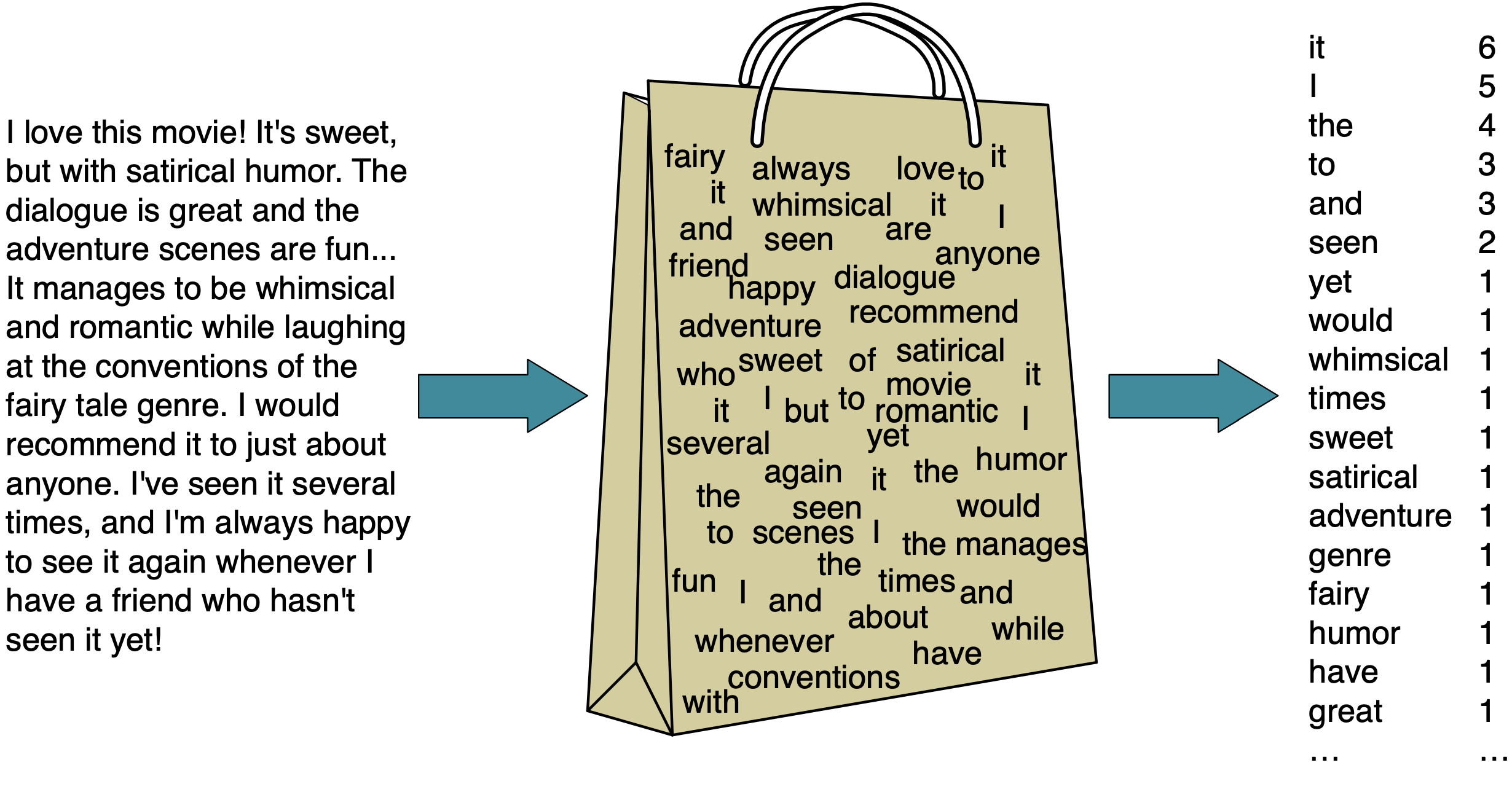
`ColumnTransformer`: Transformed data#

Adapted from here.

❓❓ Questions for you#

(iClicker) Exercise 6.1#

iClicker cloud join link: https://join.iclicker.com/SNBF

Select all of the following statements which are TRUE.

You could carry out cross-validation by passing a ColumnTransformer object to cross_validate.
After applying column transformer, the order of the columns in the transformed data has to be the same as the order of the columns in the original data.
After applying a column transformer, the transformed data is always going to be of different shape than the original data.
When you call fit_transform on a ColumnTransformer object, you get a numpy ndarray.

More on feature transformations#

`sklearn` `set_config`#

With multiple transformations in a column transformer, it can get tricky to keep track of everything happening inside it.
We can use set_config to display a diagram of this.

from sklearn import set_config

set_config(display="diagram")

ct

ColumnTransformer(transformers=[('standardscaler', StandardScaler(),
                                 ['university_years', 'lab1', 'lab3', 'lab4',
                                  'quiz1']),
                                ('passthrough', 'passthrough',
                                 ['ml_experience']),
                                ('onehotencoder', OneHotEncoder(), ['major']),
                                ('drop', 'drop',
                                 ['lab2', 'class_attendance', 'enjoy_course'])])

In a Jupyter environment, please rerun this cell to show the HTML representation or trust the notebook.
On GitHub, the HTML representation is unable to render, please try loading this page with nbviewer.org.

print(ct)

ColumnTransformer(transformers=[('standardscaler', StandardScaler(),
                                 ['university_years', 'lab1', 'lab3', 'lab4',
                                  'quiz1']),
                                ('passthrough', 'passthrough',
                                 ['ml_experience']),
                                ('onehotencoder', OneHotEncoder(), ['major']),
                                ('drop', 'drop',
                                 ['lab2', 'class_attendance', 'enjoy_course'])])

Multiple transformations in a transformer#

Recall that lab2 has missing values.

X.head(10)

	enjoy_course	ml_experience	major	class_attendance	university_years	lab1	lab2	lab3	lab4	quiz1
0	yes	1	Computer Science	Excellent	3	92	93.0	84	91	92
1	yes	1	Mechanical Engineering	Average	2	94	90.0	80	83	91
2	yes	0	Mathematics	Poor	3	78	85.0	83	80	80
3	no	0	Mathematics	Excellent	3	91	NaN	92	91	89
4	yes	0	Psychology	Good	4	77	83.0	90	92	85
5	no	1	Economics	Good	5	70	73.0	68	74	71
6	yes	1	Computer Science	Excellent	4	80	88.0	89	88	91
7	no	0	Mechanical Engineering	Poor	3	95	93.0	69	79	75
8	no	0	Linguistics	Average	2	97	90.0	94	82	80
9	yes	1	Mathematics	Average	4	95	82.0	94	94	85

So we would like to apply more than one transformations on it: imputation and scaling.
We can treat lab2 separately, but we can also include it into numeric_feats and apply both transformations on all numeric columns.

numeric_feats = [
    "university_years",
    "lab1",
    "lab2",
    "lab3",
    "lab4",
    "quiz1",
]  # apply scaling
categorical_feats = ["major"]  # apply one-hot encoding
passthrough_feats = ["ml_experience"]  # do not apply any transformation
drop_feats = ["class_attendance", "enjoy_course"]

To apply more than one transformations we can define a pipeline inside a column transformer to chain different transformations.

ct = make_column_transformer(
    (
        make_pipeline(SimpleImputer(), StandardScaler()),
        numeric_feats,
    ),  # scaling on numeric features
    ("passthrough", passthrough_feats),  # no transformations on the binary features    
    (OneHotEncoder(), categorical_feats),  # OHE on categorical features
    ("drop", drop_feats),  # drop the drop features
)

X_transformed = ct.fit_transform(X)

column_names = (
    numeric_feats
    + passthrough_feats    
    + ct.named_transformers_["onehotencoder"].get_feature_names_out().tolist()
)
column_names

['university_years',
 'lab1',
 'lab2',
 'lab3',
 'lab4',
 'quiz1',
 'ml_experience',
 'major_Biology',
 'major_Computer Science',
 'major_Economics',
 'major_Linguistics',
 'major_Mathematics',
 'major_Mechanical Engineering',
 'major_Physics',
 'major_Psychology']

pd.DataFrame(X_transformed, columns=column_names)

	university_years	lab1	lab2	lab3	lab4	quiz1	ml_experience	major_Biology	major_Computer Science	major_Economics	major_Linguistics	major_Mathematics	major_Mechanical Engineering	major_Physics	major_Psychology
0	-0.093454	0.358913	0.893260	-0.217334	0.362700	0.840028	1.0	0.0	1.0	0.0	0.0	0.0	0.0	0.0	0.0
1	-1.074719	0.590827	0.294251	-0.614206	-0.855972	0.712198	1.0	0.0	0.0	0.0	0.0	0.0	1.0	0.0	0.0
2	-0.093454	-1.264480	-0.704099	-0.316552	-1.312974	-0.693936	0.0	0.0	0.0	0.0	0.0	1.0	0.0	0.0	0.0
3	-0.093454	0.242957	0.000000	0.576409	0.362700	0.456537	0.0	0.0	0.0	0.0	0.0	1.0	0.0	0.0	0.0
4	0.887812	-1.380436	-1.103439	0.377973	0.515034	-0.054784	0.0	0.0	0.0	0.0	0.0	0.0	0.0	0.0	1.0
5	1.869077	-2.192133	-3.100139	-1.804821	-2.226978	-1.844409	1.0	0.0	0.0	1.0	0.0	0.0	0.0	0.0	0.0
6	0.887812	-1.032566	-0.105089	0.278755	-0.094302	0.712198	1.0	0.0	1.0	0.0	0.0	0.0	0.0	0.0	0.0
7	-0.093454	0.706783	0.893260	-1.705603	-1.465308	-1.333088	0.0	0.0	0.0	0.0	0.0	0.0	1.0	0.0	0.0
8	-1.074719	0.938697	0.294251	0.774844	-1.008306	-0.693936	0.0	0.0	0.0	0.0	1.0	0.0	0.0	0.0	0.0
9	0.887812	0.706783	-1.303109	0.774844	0.819702	-0.054784	1.0	0.0	0.0	0.0	0.0	1.0	0.0	0.0	0.0
10	-0.093454	1.054653	-0.504429	0.874062	0.972036	-0.949597	0.0	0.0	0.0	0.0	0.0	0.0	0.0	0.0	1.0
11	-2.055985	0.706783	-0.105089	0.675627	0.515034	-0.054784	1.0	0.0	0.0	0.0	0.0	0.0	0.0	1.0	0.0
12	-1.074719	1.054653	1.492270	0.973280	1.581372	1.862671	1.0	0.0	0.0	0.0	0.0	0.0	0.0	1.0	0.0
13	0.887812	0.706783	1.092930	0.973280	0.972036	1.862671	0.0	0.0	0.0	0.0	0.0	0.0	1.0	0.0	0.0
14	-0.093454	0.706783	0.294251	0.675627	0.972036	-1.972240	0.0	0.0	0.0	0.0	0.0	1.0	0.0	0.0	0.0
15	-0.093454	0.358913	-0.704099	-1.904039	0.819702	0.840028	1.0	0.0	1.0	0.0	0.0	0.0	0.0	0.0	0.0
16	1.869077	-1.612349	0.493921	0.675627	-0.398970	-0.054784	0.0	0.0	1.0	0.0	0.0	0.0	0.0	0.0	0.0
17	-0.093454	-0.336826	0.094581	-2.102474	-0.398970	0.200876	1.0	0.0	0.0	1.0	0.0	0.0	0.0	0.0	0.0
18	-1.074719	0.242957	0.000000	0.377973	-0.094302	-0.438275	1.0	1.0	0.0	0.0	0.0	0.0	0.0	0.0	0.0
19	-1.074719	-1.380436	1.092930	0.080319	-1.160640	0.456537	0.0	0.0	0.0	0.0	0.0	0.0	0.0	0.0	1.0
20	0.887812	0.822740	0.693590	0.576409	1.124370	0.200876	1.0	0.0	0.0	0.0	1.0	0.0	0.0	0.0	0.0

Incorporating ordinal feature `class_attendance`#

The class_attendance column is different than the major column in that there is some ordering of the values.
- Excellent > Good > Average > poor

X.head()

	enjoy_course	ml_experience	major	class_attendance	university_years	lab1	lab2	lab3	lab4	quiz1
0	yes	1	Computer Science	Excellent	3	92	93.0	84	91	92
1	yes	1	Mechanical Engineering	Average	2	94	90.0	80	83	91
2	yes	0	Mathematics	Poor	3	78	85.0	83	80	80
3	no	0	Mathematics	Excellent	3	91	NaN	92	91	89
4	yes	0	Psychology	Good	4	77	83.0	90	92	85

Let’s try applying OrdinalEncoder on this column.

X_toy = X[["class_attendance"]]
enc = OrdinalEncoder()
enc.fit(X_toy)
X_toy_ord = enc.transform(X_toy)
df = pd.DataFrame(
    data=X_toy_ord,
    columns=["class_attendance_enc"],
    index=X_toy.index,
)

pd.concat([X_toy, df], axis=1).head(10)

	class_attendance	class_attendance_enc
0	Excellent	1.0
1	Average	0.0
2	Poor	3.0
3	Excellent	1.0
4	Good	2.0
5	Good	2.0
6	Excellent	1.0
7	Poor	3.0
8	Average	0.0
9	Average	0.0

What’s the problem here?
- The encoder doesn’t know the order.
We can examine unique categories manually, order them based on our intuitions, and then provide this human knowledge to the transformer.

What are the unique categories of class_attendance?

X_toy["class_attendance"].unique()

array(['Excellent', 'Average', 'Poor', 'Good'], dtype=object)

Let’s order them manually.

class_attendance_levels = ["Poor", "Average", "Good", "Excellent"]

Note

Note that if you use the reverse order of the categories, it wouldn’t matter.

Let’s make sure that we have included all categories in our manual ordering.

assert set(class_attendance_levels) == set(X_toy["class_attendance"].unique())

oe = OrdinalEncoder(categories=[class_attendance_levels], dtype=int)
oe.fit(X_toy[["class_attendance"]])
ca_transformed = oe.transform(X_toy[["class_attendance"]])
df = pd.DataFrame(
    data=ca_transformed, columns=["class_attendance_enc"], index=X_toy.index
)
print(oe.categories_)
pd.concat([X_toy, df], axis=1).head(10)

[array(['Poor', 'Average', 'Good', 'Excellent'], dtype=object)]

	class_attendance	class_attendance_enc
0	Excellent	3
1	Average	1
2	Poor	0
3	Excellent	3
4	Good	2
5	Good	2
6	Excellent	3
7	Poor	0
8	Average	1
9	Average	1

The encoded categories are looking better now!

More than one ordinal columns?#

We can pass the manually ordered categories when we create an OrdinalEncoder object as a list of lists.
If you have more than one ordinal columns
- manually create a list of ordered categories for each column
- pass a list of lists to OrdinalEncoder, where each inner list corresponds to manually created list of ordered categories for a corresponding ordinal column.

Now let’s incorporate ordinal encoding of class_attendance in our column transformer.

	enjoy_course	ml_experience	major	class_attendance	university_years	lab1	lab2	lab3	lab4	quiz1
0	yes	1	Computer Science	Excellent	3	92	93.0	84	91	92
1	yes	1	Mechanical Engineering	Average	2	94	90.0	80	83	91
2	yes	0	Mathematics	Poor	3	78	85.0	83	80	80
3	no	0	Mathematics	Excellent	3	91	NaN	92	91	89
4	yes	0	Psychology	Good	4	77	83.0	90	92	85
5	no	1	Economics	Good	5	70	73.0	68	74	71
6	yes	1	Computer Science	Excellent	4	80	88.0	89	88	91
7	no	0	Mechanical Engineering	Poor	3	95	93.0	69	79	75
8	no	0	Linguistics	Average	2	97	90.0	94	82	80
9	yes	1	Mathematics	Average	4	95	82.0	94	94	85
10	yes	0	Psychology	Good	3	98	86.0	95	95	78
11	yes	1	Physics	Average	1	95	88.0	93	92	85
12	yes	1	Physics	Excellent	2	98	96.0	96	99	100
13	yes	0	Mechanical Engineering	Excellent	4	95	94.0	96	95	100
14	no	0	Mathematics	Poor	3	95	90.0	93	95	70
15	no	1	Computer Science	Good	3	92	85.0	67	94	92
16	yes	0	Computer Science	Average	5	75	91.0	93	86	85
17	yes	1	Economics	Average	3	86	89.0	65	86	87
18	no	1	Biology	Good	2	91	NaN	90	88	82
19	no	0	Psychology	Poor	2	77	94.0	87	81	89
20	yes	1	Linguistics	Excellent	4	96	92.0	92	96	87

numeric_feats = [
    "university_years",
    "lab1",
    "lab2",
    "lab3",
    "lab4",
    "quiz1",
]  # apply scaling
categorical_feats = ["major"]  # apply one-hot encoding
ordinal_feats = ["class_attendance"]  # apply ordinal encoding
passthrough_feats = ["ml_experience"]  # do not apply any transformation
drop_feats = ["enjoy_course"]  # do not include these features

ct = make_column_transformer(
    (
        make_pipeline(SimpleImputer(), StandardScaler()),
        numeric_feats,
    ),  # scaling on numeric features
    (
        OrdinalEncoder(categories=[class_attendance_levels], dtype=int),
        ordinal_feats,
    ),  # Ordinal encoding on ordinal features
    ("passthrough", passthrough_feats),  # no transformations on the binary features
    (OneHotEncoder(), categorical_feats),  # OHE on categorical features    
    ("drop", drop_feats),  # drop the drop features
)

X_transformed = ct.fit_transform(X)

column_names = (
    numeric_feats
    + ordinal_feats
    + passthrough_feats    
    + ct.named_transformers_["onehotencoder"].get_feature_names_out().tolist()
)
column_names

['university_years',
 'lab1',
 'lab2',
 'lab3',
 'lab4',
 'quiz1',
 'class_attendance',
 'ml_experience',
 'major_Biology',
 'major_Computer Science',
 'major_Economics',
 'major_Linguistics',
 'major_Mathematics',
 'major_Mechanical Engineering',
 'major_Physics',
 'major_Psychology']

pd.DataFrame(X_transformed, columns=column_names)

	university_years	lab1	lab2	lab3	lab4	quiz1	class_attendance	ml_experience	major_Biology	major_Computer Science	major_Economics	major_Linguistics	major_Mathematics	major_Mechanical Engineering	major_Physics	major_Psychology
0	-0.093454	0.358913	0.893260	-0.217334	0.362700	0.840028	3.0	1.0	0.0	1.0	0.0	0.0	0.0	0.0	0.0	0.0
1	-1.074719	0.590827	0.294251	-0.614206	-0.855972	0.712198	1.0	1.0	0.0	0.0	0.0	0.0	0.0	1.0	0.0	0.0
2	-0.093454	-1.264480	-0.704099	-0.316552	-1.312974	-0.693936	0.0	0.0	0.0	0.0	0.0	0.0	1.0	0.0	0.0	0.0
3	-0.093454	0.242957	0.000000	0.576409	0.362700	0.456537	3.0	0.0	0.0	0.0	0.0	0.0	1.0	0.0	0.0	0.0
4	0.887812	-1.380436	-1.103439	0.377973	0.515034	-0.054784	2.0	0.0	0.0	0.0	0.0	0.0	0.0	0.0	0.0	1.0
5	1.869077	-2.192133	-3.100139	-1.804821	-2.226978	-1.844409	2.0	1.0	0.0	0.0	1.0	0.0	0.0	0.0	0.0	0.0
6	0.887812	-1.032566	-0.105089	0.278755	-0.094302	0.712198	3.0	1.0	0.0	1.0	0.0	0.0	0.0	0.0	0.0	0.0
7	-0.093454	0.706783	0.893260	-1.705603	-1.465308	-1.333088	0.0	0.0	0.0	0.0	0.0	0.0	0.0	1.0	0.0	0.0
8	-1.074719	0.938697	0.294251	0.774844	-1.008306	-0.693936	1.0	0.0	0.0	0.0	0.0	1.0	0.0	0.0	0.0	0.0
9	0.887812	0.706783	-1.303109	0.774844	0.819702	-0.054784	1.0	1.0	0.0	0.0	0.0	0.0	1.0	0.0	0.0	0.0
10	-0.093454	1.054653	-0.504429	0.874062	0.972036	-0.949597	2.0	0.0	0.0	0.0	0.0	0.0	0.0	0.0	0.0	1.0
11	-2.055985	0.706783	-0.105089	0.675627	0.515034	-0.054784	1.0	1.0	0.0	0.0	0.0	0.0	0.0	0.0	1.0	0.0
12	-1.074719	1.054653	1.492270	0.973280	1.581372	1.862671	3.0	1.0	0.0	0.0	0.0	0.0	0.0	0.0	1.0	0.0
13	0.887812	0.706783	1.092930	0.973280	0.972036	1.862671	3.0	0.0	0.0	0.0	0.0	0.0	0.0	1.0	0.0	0.0
14	-0.093454	0.706783	0.294251	0.675627	0.972036	-1.972240	0.0	0.0	0.0	0.0	0.0	0.0	1.0	0.0	0.0	0.0
15	-0.093454	0.358913	-0.704099	-1.904039	0.819702	0.840028	2.0	1.0	0.0	1.0	0.0	0.0	0.0	0.0	0.0	0.0
16	1.869077	-1.612349	0.493921	0.675627	-0.398970	-0.054784	1.0	0.0	0.0	1.0	0.0	0.0	0.0	0.0	0.0	0.0
17	-0.093454	-0.336826	0.094581	-2.102474	-0.398970	0.200876	1.0	1.0	0.0	0.0	1.0	0.0	0.0	0.0	0.0	0.0
18	-1.074719	0.242957	0.000000	0.377973	-0.094302	-0.438275	2.0	1.0	1.0	0.0	0.0	0.0	0.0	0.0	0.0	0.0
19	-1.074719	-1.380436	1.092930	0.080319	-1.160640	0.456537	0.0	0.0	0.0	0.0	0.0	0.0	0.0	0.0	0.0	1.0
20	0.887812	0.822740	0.693590	0.576409	1.124370	0.200876	3.0	1.0	0.0	0.0	0.0	1.0	0.0	0.0	0.0	0.0

Dealing with unknown categories#

Let’s create a pipeline with the column transformer and pass it to cross_validate.

pipe = make_pipeline(ct, SVC())

scores = cross_validate(pipe, X, y, return_train_score=True)
pd.DataFrame(scores)

/Users/kvarada/miniconda3/envs/cpsc330/lib/python3.10/site-packages/sklearn/model_selection/_validation.py:821: UserWarning: Scoring failed. The score on this train-test partition for these parameters will be set to nan. Details: 
Traceback (most recent call last):
  File "/Users/kvarada/miniconda3/envs/cpsc330/lib/python3.10/site-packages/sklearn/model_selection/_validation.py", line 810, in _score
    scores = scorer(estimator, X_test, y_test)
  File "/Users/kvarada/miniconda3/envs/cpsc330/lib/python3.10/site-packages/sklearn/metrics/_scorer.py", line 527, in __call__
    return estimator.score(*args, **kwargs)
  File "/Users/kvarada/miniconda3/envs/cpsc330/lib/python3.10/site-packages/sklearn/pipeline.py", line 756, in score
    Xt = transform.transform(Xt)
  File "/Users/kvarada/miniconda3/envs/cpsc330/lib/python3.10/site-packages/sklearn/utils/_set_output.py", line 157, in wrapped
    data_to_wrap = f(self, X, *args, **kwargs)
  File "/Users/kvarada/miniconda3/envs/cpsc330/lib/python3.10/site-packages/sklearn/compose/_column_transformer.py", line 827, in transform
    Xs = self._fit_transform(
  File "/Users/kvarada/miniconda3/envs/cpsc330/lib/python3.10/site-packages/sklearn/compose/_column_transformer.py", line 681, in _fit_transform
    return Parallel(n_jobs=self.n_jobs)(
  File "/Users/kvarada/miniconda3/envs/cpsc330/lib/python3.10/site-packages/sklearn/utils/parallel.py", line 65, in __call__
    return super().__call__(iterable_with_config)
  File "/Users/kvarada/miniconda3/envs/cpsc330/lib/python3.10/site-packages/joblib/parallel.py", line 1863, in __call__
    return output if self.return_generator else list(output)
  File "/Users/kvarada/miniconda3/envs/cpsc330/lib/python3.10/site-packages/joblib/parallel.py", line 1792, in _get_sequential_output
    res = func(*args, **kwargs)
  File "/Users/kvarada/miniconda3/envs/cpsc330/lib/python3.10/site-packages/sklearn/utils/parallel.py", line 127, in __call__
    return self.function(*args, **kwargs)
  File "/Users/kvarada/miniconda3/envs/cpsc330/lib/python3.10/site-packages/sklearn/pipeline.py", line 940, in _transform_one
    res = transformer.transform(X)
  File "/Users/kvarada/miniconda3/envs/cpsc330/lib/python3.10/site-packages/sklearn/utils/_set_output.py", line 157, in wrapped
    data_to_wrap = f(self, X, *args, **kwargs)
  File "/Users/kvarada/miniconda3/envs/cpsc330/lib/python3.10/site-packages/sklearn/preprocessing/_encoders.py", line 1027, in transform
    X_int, X_mask = self._transform(
  File "/Users/kvarada/miniconda3/envs/cpsc330/lib/python3.10/site-packages/sklearn/preprocessing/_encoders.py", line 200, in _transform
    raise ValueError(msg)
ValueError: Found unknown categories ['Biology'] in column 0 during transform

  warnings.warn(

	fit_time	score_time	test_score	train_score
0	0.004824	0.002248	1.00	0.937500
1	0.004130	0.001993	1.00	0.941176
2	0.004073	0.001976	0.50	1.000000
3	0.004081	0.002009	0.75	0.941176
4	0.004038	0.006787	NaN	1.000000

What’s going on here??
Let’s look at the error message: ValueError: Found unknown categories ['Biology'] in column 0 during transform

X["major"].value_counts()

major
Computer Science          4
Mathematics               4
Mechanical Engineering    3
Psychology                3
Economics                 2
Linguistics               2
Physics                   2
Biology                   1
Name: count, dtype: int64

There is only one instance of Biology.
During cross-validation, this is getting put into the validation split.
By default, OneHotEncoder throws an error because you might want to know about this.

Simplest fix:

Pass handle_unknown="ignore" argument to OneHotEncoder
It creates a row with all zeros.

ct = make_column_transformer(
    (
        make_pipeline(SimpleImputer(), StandardScaler()),
        numeric_feats,
    ),  # scaling on numeric features
    (
        OrdinalEncoder(categories=[class_attendance_levels], dtype=int),
        ordinal_feats,
    ),  # Ordinal encoding on ordinal features
    ("passthrough", passthrough_feats),  # no transformations on the binary features
    (
        OneHotEncoder(handle_unknown="ignore"),
        categorical_feats,
    ),  # OHE on categorical features    
    ("drop", drop_feats),  # drop the drop features
)

pipe = make_pipeline(ct, SVC())

scores = cross_validate(pipe, X, y, cv=5, return_train_score=True)
pd.DataFrame(scores)

	fit_time	score_time	test_score	train_score
0	0.005081	0.002168	1.00	0.937500
1	0.004136	0.002032	1.00	0.941176
2	0.004096	0.001984	0.50	1.000000
3	0.004037	0.001962	0.75	0.941176
4	0.004015	0.001983	0.75	1.000000

With this approach, all unknown categories will be represented with all zeros and cross-validation is running OK now.

Ask yourself the following questions when you work with categorical variables

Do you want this behaviour?
Are you expecting to get many unknown categories? Do you want to be able to distinguish between them?

Cases where it’s OK to break the golden rule#

If it’s some fix number of categories. For example, if it’s something like provinces in Canada or majors taught at UBC. We know the categories in advance and this is one of the cases where it might be OK to violate the golden rule and get a list of all possible values for the categorical variable.

Categorical features with only two possible categories#

Sometimes you have features with only two possible categories.
If we apply OheHotEncoder on such columns, it’ll create two columns, which seems wasteful, as we could represent all information in the column in just one column with say 0’s and 1’s with presence of absence of one of the categories.
You can pass drop="if_binary" argument to OneHotEncoder in order to create only one column in such scenario.

X["enjoy_course"].head()

  yes
  yes
  yes
   no
  yes
Name: enjoy_course, dtype: object

ohe_enc = OneHotEncoder(drop="if_binary", dtype=int, sparse_output=False)
ohe_enc.fit(X[["enjoy_course"]])
transformed = ohe_enc.transform(X[["enjoy_course"]])
df = pd.DataFrame(data=transformed, columns=["enjoy_course_enc"], index=X.index)
pd.concat([X[["enjoy_course"]], df], axis=1).head(10)

	enjoy_course	enjoy_course_enc
0	yes	1
1	yes	1
2	yes	1
3	no	0
4	yes	1
5	no	0
6	yes	1
7	no	0
8	no	0
9	yes	1

numeric_feats = [
    "university_years",
    "lab1",
    "lab2",
    "lab3",
    "lab4",
    "quiz1",
]  # apply scaling
categorical_feats = ["major"]  # apply one-hot encoding
ordinal_feats = ["class_attendance"]  # apply ordinal encoding
binary_feats = ["enjoy_course"]  # apply one-hot encoding with drop="if_binary"
passthrough_feats = ["ml_experience"]  # do not apply any transformation
drop_feats = []

ct = make_column_transformer(
    (
        make_pipeline(SimpleImputer(), StandardScaler()),
        numeric_feats,
    ),  # scaling on numeric features
    (
        OrdinalEncoder(categories=[class_attendance_levels], dtype=int),
        ordinal_feats,
    ),  # Ordinal encoding on ordinal features
    (
        OneHotEncoder(drop="if_binary", dtype=int),
        binary_feats,
    ),  # OHE on categorical features
    ("passthrough", passthrough_feats),  # no transformations on the binary features    
    (
        OneHotEncoder(handle_unknown="ignore"),
        categorical_feats,
    ),  # OHE on categorical features
)

pipe = make_pipeline(ct, SVC())

scores = cross_validate(pipe, X, y, cv=5, return_train_score=True)
pd.DataFrame(scores)

	fit_time	score_time	test_score	train_score
0	0.005147	0.002433	1.00	1.000000
1	0.004638	0.002415	1.00	0.941176
2	0.004627	0.002340	0.50	1.000000
3	0.004699	0.002340	1.00	0.941176
4	0.004617	0.002342	0.75	1.000000

Note

Do not read too much into the scores, as we are running cross-validation on a very small dataset with 21 examples. The main point here is to show you how can we use ColumnTransformer to apply different transformations on different columns.

Break (5 min)#

`ColumnTransformer` on the California housing dataset#

housing_df = pd.read_csv("data/housing.csv")
train_df, test_df = train_test_split(housing_df, test_size=0.1, random_state=123)

train_df.head()

	longitude	latitude	housing_median_age	total_rooms	total_bedrooms	population	households	median_income	median_house_value	ocean_proximity
6051	-117.75	34.04	22.0	2948.0	636.0	2600.0	602.0	3.1250	113600.0	INLAND
20113	-119.57	37.94	17.0	346.0	130.0	51.0	20.0	3.4861	137500.0	INLAND
14289	-117.13	32.74	46.0	3355.0	768.0	1457.0	708.0	2.6604	170100.0	NEAR OCEAN
13665	-117.31	34.02	18.0	1634.0	274.0	899.0	285.0	5.2139	129300.0	INLAND
14471	-117.23	32.88	18.0	5566.0	1465.0	6303.0	1458.0	1.8580	205000.0	NEAR OCEAN

Some column values are mean/median but some are not.

Let’s add some new features to the dataset which could help predicting the target: median_house_value.

train_df = train_df.assign(
    rooms_per_household=train_df["total_rooms"] / train_df["households"]
)
test_df = test_df.assign(
    rooms_per_household=test_df["total_rooms"] / test_df["households"]
)

train_df = train_df.assign(
    bedrooms_per_household=train_df["total_bedrooms"] / train_df["households"]
)
test_df = test_df.assign(
    bedrooms_per_household=test_df["total_bedrooms"] / test_df["households"]
)

train_df = train_df.assign(
    population_per_household=train_df["population"] / train_df["households"]
)
test_df = test_df.assign(
    population_per_household=test_df["population"] / test_df["households"]
)

train_df.head()

	longitude	latitude	housing_median_age	total_rooms	total_bedrooms	population	households	median_income	median_house_value	ocean_proximity	rooms_per_household	bedrooms_per_household	population_per_household
6051	-117.75	34.04	22.0	2948.0	636.0	2600.0	602.0	3.1250	113600.0	INLAND	4.897010	1.056478	4.318937
20113	-119.57	37.94	17.0	346.0	130.0	51.0	20.0	3.4861	137500.0	INLAND	17.300000	6.500000	2.550000
14289	-117.13	32.74	46.0	3355.0	768.0	1457.0	708.0	2.6604	170100.0	NEAR OCEAN	4.738701	1.084746	2.057910
13665	-117.31	34.02	18.0	1634.0	274.0	899.0	285.0	5.2139	129300.0	INLAND	5.733333	0.961404	3.154386
14471	-117.23	32.88	18.0	5566.0	1465.0	6303.0	1458.0	1.8580	205000.0	NEAR OCEAN	3.817558	1.004801	4.323045

# Let's keep both numeric and categorical columns in the data.
X_train = train_df.drop(columns=["median_house_value", "total_rooms", "total_bedrooms", "population"])
y_train = train_df["median_house_value"]

X_test = test_df.drop(columns=["median_house_value", "total_rooms", "total_bedrooms", "population"])
y_test = test_df["median_house_value"]

from sklearn.compose import ColumnTransformer, make_column_transformer

X_train.head(10)

	longitude	latitude	housing_median_age	households	median_income	ocean_proximity	rooms_per_household	bedrooms_per_household	population_per_household
6051	-117.75	34.04	22.0	602.0	3.1250	INLAND	4.897010	1.056478	4.318937
20113	-119.57	37.94	17.0	20.0	3.4861	INLAND	17.300000	6.500000	2.550000
14289	-117.13	32.74	46.0	708.0	2.6604	NEAR OCEAN	4.738701	1.084746	2.057910
13665	-117.31	34.02	18.0	285.0	5.2139	INLAND	5.733333	0.961404	3.154386
14471	-117.23	32.88	18.0	1458.0	1.8580	NEAR OCEAN	3.817558	1.004801	4.323045
9730	-121.74	36.79	16.0	611.0	4.3814	<1H OCEAN	6.286416	1.014730	2.944354
14690	-117.09	32.80	36.0	360.0	4.7188	NEAR OCEAN	6.008333	1.019444	2.541667
7938	-118.11	33.86	33.0	393.0	5.3889	<1H OCEAN	6.078880	1.043257	3.127226
18365	-122.12	37.28	21.0	56.0	5.8691	<1H OCEAN	6.232143	1.142857	2.660714
10931	-117.91	33.74	25.0	922.0	2.9926	<1H OCEAN	4.634490	1.046638	3.195228

X_train.columns

Index(['longitude', 'latitude', 'housing_median_age', 'households',
       'median_income', 'ocean_proximity', 'rooms_per_household',
       'bedrooms_per_household', 'population_per_household'],
      dtype='object')

# Identify the categorical and numeric columns
numeric_features = [
    "longitude",
    "latitude",
    "housing_median_age",
    "households",
    "median_income",
    "rooms_per_household",
    "bedrooms_per_household",
    "population_per_household",
]

categorical_features = ["ocean_proximity"]
target = "median_income"

Let’s create a ColumnTransformer for our dataset.

X_train.info()

<class 'pandas.core.frame.DataFrame'>
Index: 18576 entries, 6051 to 19966
Data columns (total 9 columns):
 #   Column                    Non-Null Count  Dtype  
---  ------                    --------------  -----  
 0   longitude                 18576 non-null  float64
 1   latitude                  18576 non-null  float64
 2   housing_median_age        18576 non-null  float64
 3   households                18576 non-null  float64
 4   median_income             18576 non-null  float64
 5   ocean_proximity           18576 non-null  object 
 6   rooms_per_household       18576 non-null  float64
 7   bedrooms_per_household    18391 non-null  float64
 8   population_per_household  18576 non-null  float64
dtypes: float64(8), object(1)
memory usage: 1.4+ MB

X_train["ocean_proximity"].value_counts()

ocean_proximity
<1H OCEAN     8221
INLAND        5915
NEAR OCEAN    2389
NEAR BAY      2046
ISLAND           5
Name: count, dtype: int64

numeric_transformer = make_pipeline(SimpleImputer(strategy="median"), StandardScaler())
categorical_transformer = OneHotEncoder(handle_unknown="ignore")

preprocessor = make_column_transformer(
    (numeric_transformer, numeric_features),
    (categorical_transformer, categorical_features),
)

preprocessor

ColumnTransformer(transformers=[('pipeline',
                                 Pipeline(steps=[('simpleimputer',
                                                  SimpleImputer(strategy='median')),
                                                 ('standardscaler',
                                                  StandardScaler())]),
                                 ['longitude', 'latitude', 'housing_median_age',
                                  'households', 'median_income',
                                  'rooms_per_household',
                                  'bedrooms_per_household',
                                  'population_per_household']),
                                ('onehotencoder',
                                 OneHotEncoder(handle_unknown='ignore'),
                                 ['ocean_proximity'])])

In a Jupyter environment, please rerun this cell to show the HTML representation or trust the notebook.
On GitHub, the HTML representation is unable to render, please try loading this page with nbviewer.org.

X_train_pp = preprocessor.fit_transform(X_train)

When we fit the preprocessor, it calls fit on all the transformers
When we transform the preprocessor, it calls transform on all the transformers.

We can get the new names of the columns that were generated by the one-hot encoding:

preprocessor

ColumnTransformer(transformers=[('pipeline',
                                 Pipeline(steps=[('simpleimputer',
                                                  SimpleImputer(strategy='median')),
                                                 ('standardscaler',
                                                  StandardScaler())]),
                                 ['longitude', 'latitude', 'housing_median_age',
                                  'households', 'median_income',
                                  'rooms_per_household',
                                  'bedrooms_per_household',
                                  'population_per_household']),
                                ('onehotencoder',
                                 OneHotEncoder(handle_unknown='ignore'),
                                 ['ocean_proximity'])])

In a Jupyter environment, please rerun this cell to show the HTML representation or trust the notebook.
On GitHub, the HTML representation is unable to render, please try loading this page with nbviewer.org.

preprocessor.named_transformers_["onehotencoder"].get_feature_names_out(
    categorical_features
)

array(['ocean_proximity_<1H OCEAN', 'ocean_proximity_INLAND',
       'ocean_proximity_ISLAND', 'ocean_proximity_NEAR BAY',
       'ocean_proximity_NEAR OCEAN'], dtype=object)

Combining this with the numeric feature names gives us all the column names:

column_names = numeric_features + list(
    preprocessor.named_transformers_["onehotencoder"].get_feature_names_out(
        categorical_features
    )
)
column_names

['longitude',
 'latitude',
 'housing_median_age',
 'households',
 'median_income',
 'rooms_per_household',
 'bedrooms_per_household',
 'population_per_household',
 'ocean_proximity_<1H OCEAN',
 'ocean_proximity_INLAND',
 'ocean_proximity_ISLAND',
 'ocean_proximity_NEAR BAY',
 'ocean_proximity_NEAR OCEAN']

Let’s visualize the preprocessed training data as a dataframe.

pd.DataFrame(X_train_pp, columns=column_names)

	longitude	latitude	housing_median_age	households	median_income	rooms_per_household	bedrooms_per_household	population_per_household	ocean_proximity_<1H OCEAN	ocean_proximity_INLAND	ocean_proximity_ISLAND	ocean_proximity_NEAR BAY	ocean_proximity_NEAR OCEAN
0	0.908140	-0.743917	-0.526078	0.266135	-0.389736	-0.210591	-0.083813	0.126398	0.0	1.0	0.0	0.0	0.0
1	-0.002057	1.083123	-0.923283	-1.253312	-0.198924	4.726412	11.166631	-0.050132	0.0	1.0	0.0	0.0	0.0
2	1.218207	-1.352930	1.380504	0.542873	-0.635239	-0.273606	-0.025391	-0.099240	0.0	0.0	0.0	0.0	1.0
3	1.128188	-0.753286	-0.843842	-0.561467	0.714077	0.122307	-0.280310	0.010183	0.0	1.0	0.0	0.0	0.0
4	1.168196	-1.287344	-0.843842	2.500924	-1.059242	-0.640266	-0.190617	0.126808	0.0	0.0	0.0	0.0	1.0
...	...	...	...	...	...	...	...	...	...	...	...	...	...
18571	0.733102	-0.804818	0.586095	-0.966131	-0.118182	0.063110	-0.099558	0.071541	1.0	0.0	0.0	0.0	0.0
18572	1.163195	-1.057793	-1.161606	0.728235	0.357500	0.235096	-0.163397	0.007458	1.0	0.0	0.0	0.0	0.0
18573	-1.097293	0.797355	-1.876574	0.514155	0.934269	0.211892	-0.135305	0.044029	1.0	0.0	0.0	0.0	0.0
18574	-1.437367	1.008167	1.221622	-0.454427	0.006578	-0.273382	-0.149822	-0.132875	0.0	0.0	0.0	1.0	0.0
18575	0.242996	0.272667	-0.684960	-0.396991	-0.711754	0.025998	0.042957	0.051269	0.0	1.0	0.0	0.0	0.0

18576 rows × 13 columns

results_dict = {}
dummy = DummyRegressor()
results_dict["dummy"] = mean_std_cross_val_scores(
    dummy, X_train, y_train, return_train_score=True
)
pd.DataFrame(results_dict).T

	fit_time	score_time	test_score	train_score
dummy	0.001 (+/- 0.000)	0.000 (+/- 0.000)	-0.001 (+/- 0.001)	0.000 (+/- 0.000)

from sklearn.svm import SVR

knn_pipe = make_pipeline(preprocessor, KNeighborsRegressor())

knn_pipe

Pipeline(steps=[('columntransformer',
                 ColumnTransformer(transformers=[('pipeline',
                                                  Pipeline(steps=[('simpleimputer',
                                                                   SimpleImputer(strategy='median')),
                                                                  ('standardscaler',
                                                                   StandardScaler())]),
                                                  ['longitude', 'latitude',
                                                   'housing_median_age',
                                                   'households',
                                                   'median_income',
                                                   'rooms_per_household',
                                                   'bedrooms_per_household',
                                                   'population_per_household']),
                                                 ('onehotencoder',
                                                  OneHotEncoder(handle_unknown='ignore'),
                                                  ['ocean_proximity'])])),
                ('kneighborsregressor', KNeighborsRegressor())])

In a Jupyter environment, please rerun this cell to show the HTML representation or trust the notebook.
On GitHub, the HTML representation is unable to render, please try loading this page with nbviewer.org.

Pipeline

Pipeline(steps=[('columntransformer',
                 ColumnTransformer(transformers=[('pipeline',
                                                  Pipeline(steps=[('simpleimputer',
                                                                   SimpleImputer(strategy='median')),
                                                                  ('standardscaler',
                                                                   StandardScaler())]),
                                                  ['longitude', 'latitude',
                                                   'housing_median_age',
                                                   'households',
                                                   'median_income',
                                                   'rooms_per_household',
                                                   'bedrooms_per_household',
                                                   'population_per_household']),
                                                 ('onehotencoder',
                                                  OneHotEncoder(handle_unknown='ignore'),
                                                  ['ocean_proximity'])])),
                ('kneighborsregressor', KNeighborsRegressor())])

columntransformer: ColumnTransformer

ColumnTransformer(transformers=[('pipeline',
                                 Pipeline(steps=[('simpleimputer',
                                                  SimpleImputer(strategy='median')),
                                                 ('standardscaler',
                                                  StandardScaler())]),
                                 ['longitude', 'latitude', 'housing_median_age',
                                  'households', 'median_income',
                                  'rooms_per_household',
                                  'bedrooms_per_household',
                                  'population_per_household']),
                                ('onehotencoder',
                                 OneHotEncoder(handle_unknown='ignore'),
                                 ['ocean_proximity'])])

pipeline

['longitude', 'latitude', 'housing_median_age', 'households', 'median_income', 'rooms_per_household', 'bedrooms_per_household', 'population_per_household']

SimpleImputer

SimpleImputer(strategy='median')

StandardScaler

StandardScaler()

onehotencoder

['ocean_proximity']

OneHotEncoder

OneHotEncoder(handle_unknown='ignore')

KNeighborsRegressor

KNeighborsRegressor()

results_dict["imp + scaling + ohe + KNN"] = mean_std_cross_val_scores(
    knn_pipe, X_train, y_train, return_train_score=True
)

pd.DataFrame(results_dict).T

	fit_time	score_time	test_score	train_score
dummy	0.001 (+/- 0.000)	0.000 (+/- 0.000)	-0.001 (+/- 0.001)	0.000 (+/- 0.000)
imp + scaling + ohe + KNN	0.023 (+/- 0.001)	0.223 (+/- 0.017)	0.706 (+/- 0.015)	0.806 (+/- 0.015)

svr_pipe = make_pipeline(preprocessor, SVR())
results_dict["imp + scaling + ohe + SVR (default)"] = mean_std_cross_val_scores(
    svr_pipe, X_train, y_train, return_train_score=True
)

pd.DataFrame(results_dict).T

The results with scikit-learn’s default SVR hyperparameters are pretty bad.

svr_C_pipe = make_pipeline(preprocessor, SVR(C=10000))
results_dict["imp + scaling + ohe + SVR (C=10000)"] = mean_std_cross_val_scores(
    svr_C_pipe, X_train, y_train, return_train_score=True
)

pd.DataFrame(results_dict).T

With a bigger value for C the results are much better. We need to carry out systematic hyperparameter optimization to get better results. (Coming up next week.)

Note that categorical features are different than free text features. Sometimes there are columns containing free text information and we we’ll look at ways to deal with them in the later part of this lecture.

OHE with many categories#

Do we have enough data for rare categories to learn anything meaningful?
How about grouping them into bigger categories?
- Example: country names into continents such as “South America” or “Asia”
Or having “other” category for rare cases?

Do we actually want to use certain features for prediction?#

Do you want to use certain features such as gender or race in prediction?
Remember that the systems you build are going to be used in some applications.
It’s extremely important to be mindful of the consequences of including certain features in your predictive model.

Preprocessing the targets?#

Generally no need for this when doing classification.
In regression it makes sense in some cases. More on this later.
sklearn is fine with categorical labels (\(y\)-values) for classification problems.

Encoding text data#

toy_spam = [
    [
        "URGENT!! As a valued network customer you have been selected to receive a £900 prize reward!",
        "spam",
    ],
    ["Lol you are always so convincing.", "non spam"],
    ["Nah I don't think he goes to usf, he lives around here though", "non spam"],
    [
        "URGENT! You have won a 1 week FREE membership in our £100000 prize Jackpot!",
        "spam",
    ],
    [
        "Had your mobile 11 months or more? U R entitled to Update to the latest colour mobiles with camera for Free! Call The Mobile Update Co FREE on 08002986030",
        "spam",
    ],
    ["Congrats! I can't wait to see you!!", "non spam"],
]
toy_df = pd.DataFrame(toy_spam, columns=["sms", "target"])

Spam/non spam toy example#

What if the feature is in the form of raw text?
The feature sms below is neither categorical nor ordinal.
How can we encode it so that we can pass it to the machine learning algorithms we have seen so far?

toy_df

What if we apply OHE?#

### DO NOT DO THIS.
enc = OneHotEncoder(sparse_output=False)
transformed = enc.fit_transform(toy_df[["sms"]])
pd.DataFrame(transformed, columns=enc.categories_)

We do not have a fixed number of categories here.
Each “category” (feature value) is likely to occur only once in the training data and we won’t learn anything meaningful if we apply one-hot encoding or ordinal encoding on this feature.

How can we encode or represent raw text data into fixed number of features so that we can learn some useful patterns from it?
This is a well studied problem in the field of Natural Language Processing (NLP), which is concerned with giving computers the ability to understand written and spoken language.
Some popular representations of raw text include:
- Bag of words
- TF-IDF
- Embedding representations

Bag of words (BOW) representation#

One of the most popular representation of raw text
Ignores the syntax and word order
It has two components:
- The vocabulary (all unique words in all documents)
- A value indicating either the presence or absence or the count of each word in the document.

Source

Extracting BOW features using `scikit-learn`#

CountVectorizer
- Converts a collection of text documents to a matrix of word counts.
- Each row represents a “document” (e.g., a text message in our example).
- Each column represents a word in the vocabulary (the set of unique words) in the training data.
- Each cell represents how often the word occurs in the document.

Note

In the Natural Language Processing (NLP) community text data is referred to as a corpus (plural: corpora). ```

from sklearn.feature_extraction.text import CountVectorizer

vec = CountVectorizer()
X_counts = vec.fit_transform(toy_df["sms"])
bow_df = pd.DataFrame(
    X_counts.toarray(), columns=vec.get_feature_names_out(), index=toy_df["sms"]
)
bow_df

type(toy_df["sms"])

Important

Note that unlike other transformers we are passing a Series object to fit_transform. For other transformers, you can define one transformer for more than one columns. But with CountVectorizer you need to define separate CountVectorizer transformers for each text column, if you have more than one text columns.

X_counts

Why sparse matrices?#

Most words do not appear in a given document.
We get massive computational savings if we only store the nonzero elements.
There is a bit of overhead, because we also need to store the locations:
- e.g. “location (3,27): 1”.
However, if the fraction of nonzero is small, this is a huge win.

print("The total number of elements: ", np.prod(X_counts.shape))
print("The number of non-zero elements: ", X_counts.nnz)
print(
    "Proportion of non-zero elements: %0.4f" % (X_counts.nnz / np.prod(X_counts.shape))
)
print(
    "The value at cell 3,%d is: %d"
    % (vec.vocabulary_["jackpot"], X_counts[3, vec.vocabulary_["jackpot"]])
)

Question for you

What would happen if you apply StandardScaler on sparse data?

`OneHotEncoder` and sparse features#

By default, OneHotEncoder also creates sparse features.
You could set sparse=False to get a regular numpy array.
If there are a huge number of categories, it may be beneficial to keep them sparse.
For smaller number of categories, it doesn’t matter much.

Important hyperparameters of `CountVectorizer`#

binary
- whether to use absence/presence feature values or counts
max_features
- only consider top max_features ordered by frequency in the corpus
max_df
- ignore features which occur in more than max_df documents
min_df
- ignore features which occur in less than min_df documents
ngram_range
- consider word sequences in the given range

Let’s look at all features, i.e., words (along with their frequencies).

vec = CountVectorizer()
X_counts = vec.fit_transform(toy_df["sms"])
bow_df = pd.DataFrame(
    X_counts.toarray(), columns=vec.get_feature_names_out(), index=toy_df["sms"]
)
bow_df

When we use binary=True, the representation uses presence/absence of words instead of word counts.

vec_binary = CountVectorizer(binary=True)
X_counts = vec_binary.fit_transform(toy_df["sms"])
bow_df = pd.DataFrame(
    X_counts.toarray(), columns=vec_binary.get_feature_names_out(), index=toy_df["sms"]
)
bow_df

We can control the size of X (the number of features) using max_features.

vec8 = CountVectorizer(max_features=8)
X_counts = vec8.fit_transform(toy_df["sms"])
bow_df = pd.DataFrame(
    X_counts.toarray(), columns=vec8.get_feature_names_out(), index=toy_df["sms"]
)
bow_df

Note

Notice that vec8 and vec8_binary have different vocabularies, which is kind of unexpected behaviour and doesn’t match the documentation of scikit-learn.

Here is the code for binary=True condition in scikit-learn. As we can see, the binarization is done before limiting the features to max_features, and so now we are actually looking at the document counts (in how many documents it occurs) rather than term count. This is not explained anywhere in the documentation.

The ties in counts between different words makes it even more confusing. I don’t think it’ll have a big impact on the results but this is good to know! Remember that scikit-learn developers are also humans who are prone to make mistakes. So it’s always a good habit to question whatever tools we use every now and then.

vec8 = CountVectorizer(max_features=8)
X_counts = vec8.fit_transform(toy_df["sms"])
pd.DataFrame(
    data=X_counts.sum(axis=0).tolist()[0],
    index=vec8.get_feature_names_out(),
    columns=["counts"],
).sort_values("counts", ascending=False)

vec8_binary = CountVectorizer(binary=True, max_features=8)
X_counts = vec8_binary.fit_transform(toy_df["sms"])
pd.DataFrame(
    data=X_counts.sum(axis=0).tolist()[0],
    index=vec8_binary.get_feature_names_out(),
    columns=["counts"],
).sort_values("counts", ascending=False)

Preprocessing#

Note that CountVectorizer is carrying out some preprocessing such as because of the default argument values
- Converting words to lowercase (lowercase=True)
- getting rid of punctuation and special characters (token_pattern ='(?u)\\b\\w\\w+\\b')

pipe = make_pipeline(CountVectorizer(), SVC())

pipe.fit(toy_df["sms"], toy_df["target"])

pipe.predict(toy_df["sms"])

Is this a realistic representation of text data?#

Of course this is not a great representation of language
- We are throwing out everything we know about language and losing a lot of information.
- It assumes that there is no syntax and compositional meaning in language.
But it works surprisingly well for many tasks.
We will learn more expressive representations in the coming weeks.

❓❓ Questions for you#

(iClicker) Exercise 6.2#

iClicker cloud join link: https://join.iclicker.com/3DP5H

Select all of the following statements which are TRUE.

(A) handle_unknown="ignore" would treat all unknown categories equally.
(B) As you increase the value for max_features hyperparameter of CountVectorizer the training score is likely to go up.
(C) Suppose you are encoding text data using CountVectorizer. If you encounter a word in the validation or the test split that’s not available in the training data, we’ll get an error.
(D) In the code below, inside cross_validate, each fold might have slightly different number of features (columns) in the fold.

pipe = (CountVectorizer(), SVC())
cross_validate(pipe, X_train, y_train)

What did we learn today?#

Motivation to use ColumnTransformer
ColumnTransformer syntax
Defining transformers with multiple transformations
How to visualize transformed features in a dataframe
More on ordinal features
Different arguments OneHotEncoder
- handle_unknow="ignore"
- if_binary
Dealing with text features
- Bag of words representation: CountVectorizer

Lecture 6: sklearn ColumnTransformer and Text Features

Contents

Lecture 6: sklearn ColumnTransformer and Text Features#

Imports, Announcements, and LO#

Imports#

Learning outcomes#

sklearn’s ColumnTransformer#

Transformations on the toy data#

ColumnTransformer example#

Data#

Identify the transformations we want to apply#

Create a column transformer#

Convenient make_column_transformer syntax#

Let’s examine the transformed data#

Viewing the transformed data as a dataframe#

ColumnTransformer: Transformed data#

Training models with transformed data#

❓❓ Questions for you#

(iClicker) Exercise 6.1#

More on feature transformations#

sklearn set_config#

Multiple transformations in a transformer#

Incorporating ordinal feature class_attendance#

More than one ordinal columns?#

Dealing with unknown categories#

Cases where it’s OK to break the golden rule#

Categorical features with only two possible categories#

Break (5 min)#

ColumnTransformer on the California housing dataset#

OHE with many categories#

Do we actually want to use certain features for prediction?#

Preprocessing the targets?#

Encoding text data#

Spam/non spam toy example#

What if we apply OHE?#

Bag of words (BOW) representation#

Extracting BOW features using scikit-learn#

Why sparse matrices?#

OneHotEncoder and sparse features#

Important hyperparameters of CountVectorizer#

Preprocessing#

Is this a realistic representation of text data?#

❓❓ Questions for you#

(iClicker) Exercise 6.2#

What did we learn today?#

Lecture 6: `sklearn` `ColumnTransformer` and Text Features#

sklearn’s `ColumnTransformer`#

`ColumnTransformer` example#

Convenient `make_column_transformer` syntax#

`ColumnTransformer`: Transformed data#

`sklearn` `set_config`#

Incorporating ordinal feature `class_attendance`#

`ColumnTransformer` on the California housing dataset#

Extracting BOW features using `scikit-learn`#

`OneHotEncoder` and sparse features#

Important hyperparameters of `CountVectorizer`#