Explain how linear models make predictions using coefficients and an intercept.
Explain intuitively how a loss function evaluates predictions and guides model fitting.
Describe the behaviour of squared-error loss and log loss, including which mistakes they penalize most strongly.
Distinguish the loss used to fit a model from the score used to evaluate it.
Fit and use Ridge for regression and LogisticRegression for classification.
Explain at a high level why linear models use regularization and how alpha and C affect model complexity.
Explain how logistic regression converts a linear score into a probability and a class prediction.
Interpret linear-model coefficients while accounting for scaling, correlated features, and the distinction between prediction and causation.
Contrast parametric linear models with a non-parametric model such as \(k\)-NN.
Describe important strengths and limitations of linear models.
In Chapter 4, \(k\)-NN made predictions by finding similar training examples. In Chapter 6, we built feature representations that could contain thousands of columns, such as word counts. Comparing a new example with the training set can become expensive as these datasets grow. Could we instead learn a compact rule that combines the features directly?
A linear model learns one coefficient per feature and an intercept. To predict, it multiplies each feature value by its coefficient, adds the contributions, and adds the intercept. Once fitted, it can predict without searching the training examples. This makes linear models useful when fast predictions or large feature representations matter.
The simplicity of this rule also limits the relationships it can represent. We will explore that trade-off through regression and classification, using familiar pipelines and cross-validation to evaluate the models. The weighted sums we develop here are also building blocks of neural networks; we will return to that connection at the end of the chapter.
Show imports and setup
from pathlib import Pathimport matplotlib.pyplot as pltimport numpy as npimport pandas as pdfrom sklearn.dummy import DummyClassifier, DummyRegressorfrom sklearn.linear_model import LogisticRegression, Ridgefrom sklearn.model_selection import cross_validate, train_test_splitfrom sklearn.neighbors import KNeighborsClassifierfrom sklearn.pipeline import make_pipelinefrom sklearn.preprocessing import StandardScalerfrom sklearn.svm import SVCDATA_DIR = Path("data")
How linear models predict and learn
What makes a model linear?
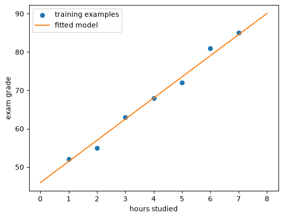
Suppose we want to predict a student’s exam grade from the number of hours they studied. A linear model represents its prediction as a line:
\[
\hat{y} = w_1x_1 + b.
\]
Here, \(x_1\) is the number of study hours, \(w_1\) is the coefficient (or weight), and \(b\) is the intercept (or bias). The coefficient tells us how much the prediction changes when the feature increases by one unit (one hour in this example).
The intercept is the model’s prediction when the feature equals zero: here, the predicted grade at zero study hours. It lets the line shift up or down instead of forcing it to pass through the origin. Whether that prediction is meaningful depends on the data; a fitted line need not be reliable at study times outside the range we observed.
study_data = pd.DataFrame( {"hours": [1, 2, 3, 4, 5, 6, 7],"grade": [52, 55, 63, 68, 72, 81, 85], })study_model = Ridge(alpha=1.0) # a commonly used linear model for regression problemsstudy_model.fit(study_data[["hours"]], study_data["grade"])hours_grid = pd.DataFrame({"hours": np.linspace(0, 8, 100)})plt.scatter(study_data["hours"], study_data["grade"], label="training examples")plt.plot( hours_grid["hours"], study_model.predict(hours_grid), color="tab:orange", label="fitted model",)plt.xlabel("hours studied")plt.ylabel("exam grade")plt.legend();
According to the fitted line, the predicted grade for a student who studies for about 5.5 hours is approximately 76%. This is a prediction from the model, not a guarantee about what the student will receive.
The model makes a strong simplifying assumption: the predicted grade changes at a constant rate as study time increases. Because the learned coefficient is positive, increasing the study-hours input always increases the predicted grade. Is that plausible for every student and any number of hours?
In reality, additional study may have diminishing benefits, excessive studying may cause fatigue, and grades depend on many factors absent from this one-feature model. The fitted line would eventually predict grades above 100% if we extrapolated far enough. Moreover, an association between study time and grades does not by itself show that additional studying causes the predicted increase.
A linear model can still be useful when a straight line is a reasonable approximation over the range where predictions will be made. The line does not need to pass through every training example. Fitting must choose a coefficient and intercept from many possible values; shortly, we will look under the hood of fit and introduce the criterion used to make that choice.
With more features, each feature makes its own contribution. Suppose a model uses hours studied and practice sets completed. For one student,
Feature
Value
Coefficient
Contribution
Hours studied (\(x_1\))
5
4
20
Practice sets (\(x_2\))
6
2
12
Intercept (\(b\))
45
so the predicted grade is \(20+12+45=77\). In general, with \(d\) features, the rule is
\[
\hat{y}=w_1x_1+w_2x_2+\cdots+w_dx_d+b.
\]
Each term is one feature’s contribution. The model uses the same coefficients for every example.
We can collect the coefficients into a vector \(\mathbf{w}\) and the feature values into a vector \(\mathbf{x}\). Their dot product, written \(\mathbf{w}^{\mathsf T}\mathbf{x}\), means multiplying corresponding entries and adding them. For the student above, it is \(4\times5+2\times6=32\). This gives us a shorter way to write the same prediction:
\[
\hat{y}=\mathbf{w}^{\mathsf T}\mathbf{x}+b.
\]
With one feature, this prediction rule describes a line; with two features, a plane; and with more features, a hyperplane. You can follow the examples in this chapter by thinking of the rule as a weighted sum.
NoteOptional: Predicting for a whole dataset
For a complete dataset, we stack the examples as rows of a feature matrix \(X\):
Each column of \(X\) is a feature, while \(\mathbf{y}\) contains the observed targets. The model applies the same coefficient vector to every row:
\[
\hat{\mathbf{y}}=X\mathbf{w}+b,
\]
where \(+b\) means adding the intercept to every prediction. You may also see the prediction written more compactly as
\[
\hat{\mathbf{y}}=X\mathbf{w},
\]
without a separate \(b\). In that convention, \(X\) contains an additional feature whose value is always 1, and the corresponding coefficient in \(\mathbf{w}\) is the intercept. Because \(1\times b=b\), this adds the intercept to every prediction. We say that the intercept has been absorbed into \(X\mathbf{w}\).
So far, we have supplied coefficients or let fit choose them. How does fitting decide which values to use?
What happens during fit?
So far, we have mostly treated a scikit-learn model as an object with a convenient interface: call fit using training data, then use the fitted model to predict and evaluate new examples. Let us briefly look inside fit.
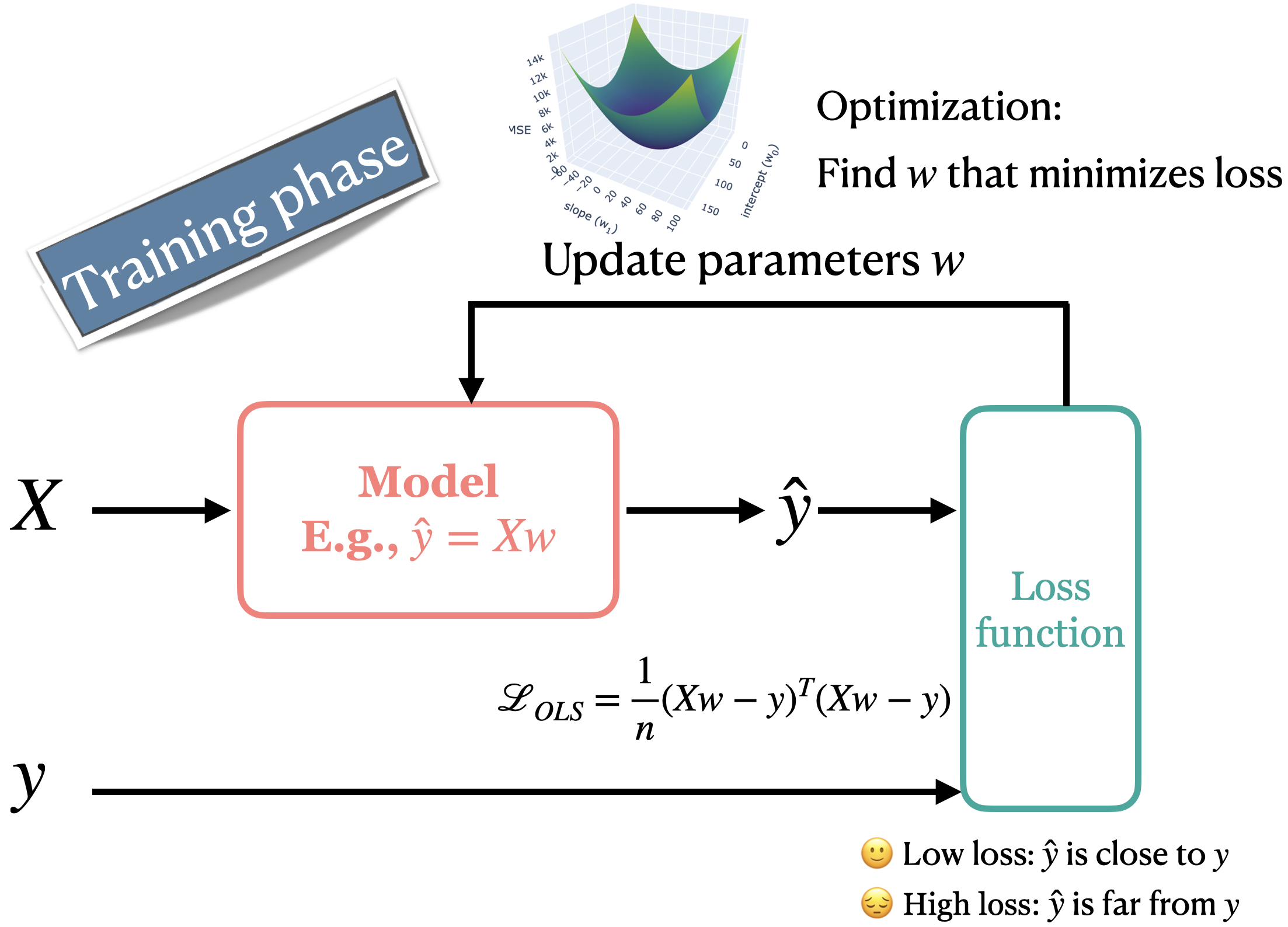
During supervised learning, a model uses the feature matrix \(X\) and its current parameters to produce predictions \(\hat{y}\). A loss function compares those predictions with the observed targets \(y\) and returns a number describing how poorly they agree. Low loss means the predictions are close to what the loss function rewards; high loss means they are not.
An optimization procedure finds parameter values that reduce the fitting objective. One common approach repeatedly evaluates predictions, measures their loss, and updates the parameters, as shown below. Some models can instead be fitted by directly solving a system of equations. Scikit-learn handles these computations when we call fit. The computational details of optimization are beyond the scope of this book; the important idea is that the loss function tells the fitting procedure what counts as a better model.
The supervised-learning training loop. A model uses features X and its current parameters to produce predictions. A loss function compares the predictions with observed targets y, and an optimization procedure updates the parameters to reduce the loss.
The choice of loss function depends on the prediction problem and on which kinds of mistakes we want the model to treat as costly. Different loss functions can therefore lead to different fitted models.
The diagram shows a common choice for regression: mean squared error. For each training example, subtract the prediction from the observed target: \(y-\hat{y}\). We will call this difference the residual. A positive residual means the model predicted too low; a negative one means it predicted too high. Mean squared error squares these residuals and takes their mean. The diagram subtracts in the opposite order, but squaring gives the same result. A large mean squared error indicates that the predictions have large squared differences from the targets, on average. A small value indicates that the predictions are closer to the targets according to this particular loss. Ordinary least squares fits a linear model by finding coefficients that minimize squared-error loss.
For example, suppose two students both receive a grade of 70, and the model predicts 68 and 66. Their residuals are 2 and 4, so their squared errors are 4 and 16. The mean squared error is \((4+16)/2=10\). Doubling the size of the error makes its contribution four times as large. Squared-error loss therefore gives especially large weight to large mistakes.
A low training loss means that the model fits its training examples well; it does not necessarily mean that the model will predict new examples well. We still need validation or cross-validation to assess generalization. Loss is also not necessarily the value reported by a model’s score method: a model can be fitted using one objective and evaluated using another measure. We will see this distinction with Ridge regression.
Linear regression with Ridge
Linear regression uses a linear prediction rule for a numeric target. In this book, we will use scikit-learn’s Ridge estimator rather than LinearRegression. Both use coefficients and an intercept to make predictions, but Ridge includes regularization, which discourages unnecessarily large coefficients. This often makes the fitted model more stable when features contain overlapping information and can reduce overfitting.
Let’s try Ridge on a housing-price prediction problem using the California housing dataset. Each row represents a census block group rather than an individual house, and the target is the median house value in that block group.
We will reuse the feature representation developed in Chapter 6. The raw room, bedroom, and population totals partly measure the size of a block group. Dividing them by the number of households produces features that are easier to compare across block groups of different sizes. These calculations use values from only one row at a time, so they do not learn information from validation or test examples.
We begin with a mean-prediction baseline. We then place StandardScaler and Ridge in a pipeline so that the scaler is fit separately within each cross-validation fold.
By default, regression estimators use \(R^2\) for their score method, so these values are not losses. The Ridge model improves substantially over always predicting the training mean. Later chapters examine regression metrics and their interpretation in more detail.
Controlling model complexity
Many sets of coefficients can fit the training data similarly, especially when features are correlated. In those situations, small changes to the training data can produce large changes in the learned coefficients. Regularization makes Ridge prefer less extreme coefficients unless larger values improve the fit enough to justify them. At a high level, this is another way to control model complexity.
NoteOptional: What Ridge minimizes
Ordinary least squares chooses coefficients by minimizing squared-error loss. Ridge adds a penalty based on the squared coefficients:
\[
\text{quantity minimized by Ridge}
=
\sum_{i=1}^{n}(y_i-\hat{y}_i)^2
+
\alpha\sum_{j=1}^{d}w_j^2.
\]
Here, \(n\) is the number of training examples. The first term is the sum of squared errors. Taking the mean instead gives the same unregularized least-squares fit, but changes the balance with the penalty unless we also adjust alpha. The intercept is not included in the penalty. The first term rewards predictions close to the training targets. The second discourages large coefficients. The optimization procedure searches for coefficients that balance these two goals. The details of that optimization are beyond the scope of this book.
The hyperparameter alpha controls the strength of regularization:
A larger alpha discourages large coefficients more strongly, usually producing a less flexible model with a greater risk of underfitting.
A smaller alpha allows the model to follow the training data more closely, usually producing a more flexible model with a greater risk of overfitting.
Regularization changes which coefficients the model prefers; it does not change the weighted-sum prediction rule or remove coefficients from the model. We use Ridge here so that we can control this preference. The appropriate value of alpha is data-dependent and can be selected using cross-validation.
Scaling matters because regularization acts on coefficient magnitudes. Without scaling, changing a feature from dollars to thousands of dollars changes the size of its coefficient and therefore how strongly that feature is affected by the penalty. This is why our Ridge pipeline includes StandardScaler.
For this dataset, the training and cross-validation scores barely change across the smaller values of alpha. At very large values, both scores fall toward the mean-prediction baseline: the penalty constrains the coefficients so strongly that the model underfits. More regularization is not always better, and a small difference between training and validation scores is not enough to establish that a model is useful.
We should not choose alpha by repeatedly checking the test set. Chapter 8 develops methods for selecting hyperparameters using only the training data.
Interpreting coefficients
After fitting the pipeline, we can inspect the coefficients learned by Ridge. Each coefficient describes how the model’s prediction changes as its corresponding feature changes, holding the other represented features fixed. Because the pipeline scales the features before fitting, their numerical scales are comparable, making their coefficient magnitudes easier to compare.
A positive coefficient means that increasing the feature, while keeping the other represented features fixed, increases the model’s prediction. A negative coefficient decreases the prediction. With StandardScaler, a one-unit increase in a scaled feature corresponds to an increase of one training-set standard deviation in the original feature. Its coefficient is therefore the change in predicted house value, in dollars, for that increase while holding the other represented features fixed. A larger absolute coefficient means a larger prediction change for this particular size of change.
That interpretation needs several qualifications:
The coefficient describes the fitted model, not necessarily how the world works. It is not a causal effect.
Correlated features can share or exchange predictive information, making individual coefficients unstable or surprising.
Without comparable scaling, coefficient magnitudes cannot be compared directly because a one-unit change means something different for each feature.
A coefficient gives a constant change per unit. If the real relationship curves or depends on another feature, that summary may be inadequate.
In this standardized pipeline, zero represents each feature’s training mean. The intercept is the prediction at that combination of means, which need not describe an actual block group.
Coefficients can help us understand how a model computes predictions, but they should be treated as evidence about the model rather than automatic feature importance or causal evidence.
In the fitted Ridge model above, median_income has a positive coefficient, whereas rooms_per_household has a negative coefficient. Does this establish that increasing the average number of rooms would lower a district’s house values? Explain what the negative coefficient says about this model’s predictions and what it does not say about the world. Consider the other features held fixed, the district-level nature of the data, and information not included in the model.
Logistic regression
Regression produces a numeric prediction directly. For classification, we instead need to choose among classes. Despite its name, logistic regression is a classifier. Like linear regression, it first computes a weighted sum:
\[
z = \mathbf{w}^{\mathsf T}\mathbf{x}+b.
\]
This value is often called the decision score or raw score. In binary classification, its sign determines which side of the decision boundary an example lies on.
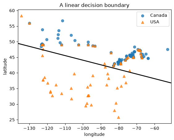
Let’s return to the Canada-USA cities classification problem from Chapter 2. The features are a city’s longitude and latitude, and the target indicates whether it is in Canada or the United States.
An aerial view of the Canada-USA border highlighted between forested areas.
Alaska is an obvious complication: geography is not truly separated by one straight line. This makes the dataset useful for studying both a linear classifier and its limitations.
We fit the pipeline to examine a prediction. The model’s classes_ attribute records the class order. In binary logistic regression, a negative decision score selects classes_[0], while a positive score selects classes_[1]. This ordering is deterministic; the model does not randomly designate the positive class.
The decision boundary contains feature values whose score is zero:
\[
\mathbf{w}^{\mathsf T}\mathbf{x}+b=0.
\]
With two features, this boundary is a line. With three, it is a plane; with \(d\) features, it is a \((d-1)\)-dimensional hyperplane. A linear classifier can still make mistakes on its training data: a linear boundary is the form of the rule, not a requirement that the classes be perfectly separable.
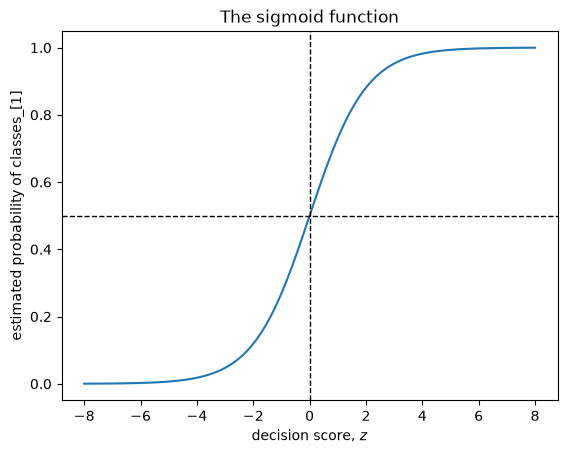
The sign of the score is enough to choose a class, but its magnitude contains additional information. Logistic regression passes the score through the sigmoid function:
\[
\sigma(z)=\frac{1}{1+e^{-z}}.
\]
The sigmoid maps any real-valued score to a number between 0 and 1. This number is the model’s estimated probability of classes_[1]. A score of zero maps to 0.5, so thresholding the probability at 0.5 is equivalent to thresholding the score at zero.
The sigmoid is a nonlinear function, but it does not bend the decision boundary: the boundary is still where the linear score equals zero. This is why logistic regression is called a linear classifier even though its predicted probability is not a linear function of the features.
decision_score = logistic_pipe.decision_function(example)[0]pd.Series( {"sigmoid(decision_score)": sigmoid(decision_score),"predict_proba for classes_[1]": logistic_pipe.predict_proba(example)[0, 1], })
sigmoid(decision_score)          0.402317
predict_proba for classes_[1]    0.402317
dtype: float64
predict_proba returns one column per class in the order given by classes_. For binary classification the two probabilities sum to one. The larger probability determines the default hard prediction, but an application may choose a different threshold when different errors have different consequences.
An estimated probability is useful, but it should not automatically be treated as trustworthy confidence. A model can assign a high probability to an incorrect prediction, particularly when its assumptions are inadequate or deployment examples differ from its training data. Later chapters discuss evaluation measures and probability calibration.
Log loss
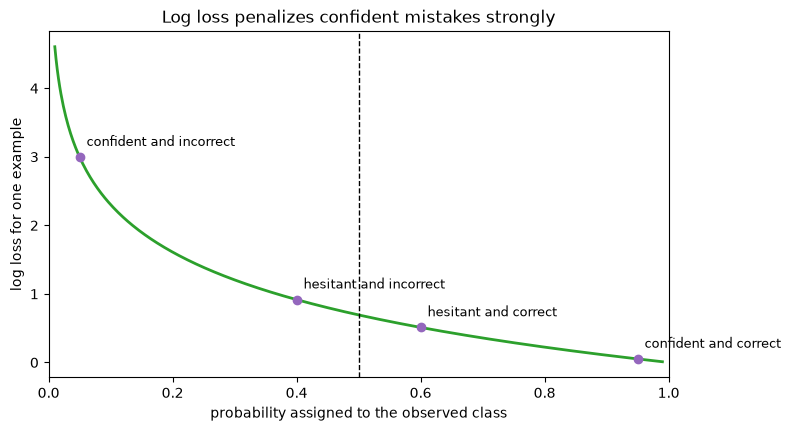
Logistic regression chooses its coefficients using log loss, also called cross-entropy loss. For one example, let \(p_{\text{observed}}\) be the probability that the model assigns to the class that was actually observed. Its loss is
\[
-\log\left(p_{\text{observed}}\right).
\]
The loss is small when the model assigns high probability to the observed class. It grows as that probability approaches zero, so a confident incorrect prediction receives a particularly large penalty. During fitting, regularized logistic regression balances log loss across the training examples against a penalty on the coefficients. As with Ridge, the aim is to fit the data without making the coefficients unnecessarily large.
probability_observed = np.linspace(0.01, 0.99, 500)example_loss =-np.log(probability_observed)case_probabilities = np.array([0.05, 0.40, 0.60, 0.95])case_labels = ["confident and incorrect","hesitant and incorrect","hesitant and correct","confident and correct",]fig, ax = plt.subplots(figsize=(8, 4.5))ax.plot(probability_observed, example_loss, color="tab:green", linewidth=2)ax.axvline(0.5, color="black", linestyle="--", linewidth=1)ax.scatter( case_probabilities,-np.log(case_probabilities), color="tab:purple", zorder=3,)for probability, label inzip(case_probabilities, case_labels): ax.annotate( label, (probability, -np.log(probability)), xytext=(5, 8), textcoords="offset points", fontsize=9, )ax.set_xlabel("probability assigned to the observed class")ax.set_ylabel("log loss for one example")ax.set_title("Log loss penalizes confident mistakes strongly")ax.set_xlim(0, 1);
With the usual 0.5 classification threshold:
Confident and correct \(\rightarrow\) very small loss
Hesitant and correct \(\rightarrow\) somewhat larger loss
Hesitant and incorrect \(\rightarrow\) larger loss
Confident and incorrect \(\rightarrow\) very large loss
Accuracy treats a probability of 0.51 and a probability of 0.99 identically when the observed class is predicted: both count as correct. Log loss distinguishes them because it considers how much probability the model assigned to the observed class.
As with Ridge, LogisticRegression minimizes its loss together with a regularization penalty. Its C hyperparameter controls regularization in the opposite direction from the alpha of Ridge:
Smaller C means stronger regularization and usually a less flexible model.
Larger C means weaker regularization and usually a more flexible model.
This reversal is easy to forget: alpha directly controls regularization strength, whereas C controls inverse regularization strength.
At the smallest values of C, both training and cross-validation accuracy are low, indicating underfitting. Accuracy improves as the penalty weakens, then changes little across the larger values. Weakening regularization further does not necessarily improve validation performance. Also, these tables report accuracy, whereas fitting uses log loss plus a penalty: probabilities can change even when the predicted classes stay the same.
Confidence and model limitations
For a linear classifier, examples close to the decision boundary have scores near zero and probabilities near 0.5. Examples far from the boundary generally receive more extreme probabilities. Distance from the boundary describes the model’s certainty under its fitted rule; it does not guarantee that the rule is correct.
The second table shows the incorrect training predictions with the highest predicted probabilities. Some cities in Alaska can be geographically far from the model’s straight boundary even though they belong to the United States. The model can therefore be confidently wrong because its linear representation cannot express the actual geography.
This is a general lesson: probability estimates are conditional on the model, its features, and the data used to fit it. A high value from predict_proba is not a guarantee.
NoteOther linear classifiers
A linear SVM uses the same weighted-sum form as logistic regression, but learns its coefficients using a different loss function. Logistic regression uses log loss and naturally provides probabilities; a linear SVM uses a margin-based loss. Their boundaries can therefore differ even on the same training data.
In scikit-learn, LinearSVC is designed specifically for linear classification, while SVC(kernel="linear") is a linear-kernel version of the SVM introduced in Chapter 4. Logistic regression will be our main linear classifier when probability estimates are useful.
When to use linear models
Recall that \(k\)-NN retains training examples and searches for neighbours when predicting. A fitted linear model instead retains coefficients and an intercept. This difference helps explain when each approach is useful.
Linear models are commonly described as parametric: once the feature representation is fixed, the prediction rule has a fixed number of learned parameters. A linear regression or binary logistic-regression model with 100 features learns 100 coefficients and an intercept whether it has 1,000 training examples or one million. By contrast, \(k\)-NN is non-parametric: its stored representation grows with the training set.
In statistics, “parametric” often describes a family of probability distributions specified by a fixed number of parameters. Here, we focus on the fixed-size prediction rule. Calling linear regression parametric does not mean that its features or target must follow a normal distribution. Fitting a least-squares prediction rule does not itself require normally distributed errors either; additional distributional assumptions arise in some statistical uses of the model. Likewise, non-parametric does not mean assumption-free: \(k\)-NN relies on nearby examples having similar targets under the chosen representation and distance.
“Non-parametric” also does not mean that a method has no hyperparameters: \(k\), the distance measure, and neighbour weighting are all choices we make. Nor does “parametric” mean small or unable to overfit. With 100,000 features, a linear regression model learns 100,001 parameters and may still overfit without enough data or regularization.
Question
Linear model
\(k\)-NN
What does fitting retain?
Coefficients and an intercept
The training examples
Where is most computation?
During fitting
During prediction
What shapes can it represent directly?
A linear function or boundary
Flexible, locally determined shapes
What happens as training rows are added?
The number of coefficients stays fixed for fixed \(d\)
Storage and straightforward prediction work grow
What assumption does it make?
A linear relationship is a useful approximation
Nearby examples tend to have similar targets
These comparisons suggest useful starting points, not guaranteed winners. Try a regularized linear model early when fast prediction matters or the feature matrix is large and sparse, as with bag-of-words. Its coefficients also make the prediction calculation relatively transparent, subject to the interpretation cautions discussed earlier. For a small dataset with useful local structure and a curved boundary, \(k\)-NN may be a better starting point. Compare validation performance and computation time before choosing.
A linear model’s central restriction concerns its represented features: linear regression assigns each feature a constant coefficient, and logistic regression uses a linear boundary. Curved relationships and interactions can be missed. Later feature-engineering techniques can supply transformed or interaction features that let a linear model represent some nonlinear relationships, although these choices introduce their own assumptions and complexity.
The weighted sum also appears inside neural networks. A neural-network layer can compute several weighted sums, each with its own coefficients and intercept, and then apply nonlinear functions to the results. Subsequent layers use those outputs as their inputs. Combining these operations allows networks to represent more complicated relationships. Simply stacking weighted sums with intercepts, without nonlinear functions between them, would still give a linear prediction rule.
Exercises
Exercise 7.1: Parametric and non-parametric models (multiple select)
Select all statements that are true.
A binary logistic-regression model trained with \(d\) features learns \(d\) coefficients and one intercept.
Increasing the number of training examples increases the number of coefficients learned by logistic regression.
A fitted \(k\)-NN model generally retains its training examples.
Calling a model non-parametric means that it has no hyperparameters.
With the same 100 input features, a binary logistic-regression model learns the same number of coefficients from 1,000 examples as it does from one million examples.
TipSolution
A, C, and E are true. For a fixed feature representation, logistic regression learns one coefficient per feature and an intercept, regardless of the number of training examples. In contrast, \(k\)-NN retains the training examples. Non-parametric models can still have hyperparameters such as \(k\).
Exercise 7.2: Trace a regression prediction and its loss
A linear model uses \(\hat y=3x+10\). Compute its predictions for \(x=2\) and \(x=5\). If the observed targets are 18 and 20, compute each residual, each squared error, and the mean squared error. Which example has more influence on the squared-error loss?
TipSolution
For \(x=2\), the prediction is 16, the residual is \(18-16=2\), and the squared error is 4. For \(x=5\), the prediction is 25, the residual is \(20-25=-5\), and the squared error is 25. The mean squared error is \((4+25)/2=14.5\). The second example has more influence because its error has the larger magnitude.
Exercise 7.3: Predict the effect of regularization
A scaled Ridge model performs well on its training data but much worse in cross-validation. A classmate proposes increasing alpha by a large amount and selecting the value with the best test score. Before running anything, explain what increasing alpha encourages the model to do. Could it help? Could it make both training and validation performance worse? How would you revise the classmate’s selection procedure? What direction would you change C to strengthen regularization in logistic regression?
TipSolution
Increasing alpha encourages smaller coefficients. This may reduce overfitting and improve validation performance, but excessive regularization can make the model underfit, worsening both training and validation performance. Select alpha using cross-validation on the training data, keeping the test set for final evaluation. For logistic regression, decrease C to strengthen regularization.
Exercise 7.4: Same accuracy, different probabilities
Two binary classifiers predict the observed class correctly for each of two examples. Model A assigns the observed class probabilities of 0.6 and 0.6; model B assigns probabilities of 0.9 and 0.9. Compare their accuracy and log loss without calculating logarithms. Now both models encounter a third example and predict the wrong class: A assigns the observed class probability 0.4, while B assigns it probability 0.01. Which model receives the larger loss on this example, and why? Does a high predicted probability guarantee correctness?
TipSolution
Both models have 100% accuracy on the first two examples, but B has lower log loss because it assigns higher probabilities to the observed classes. On the third example, B receives a much larger loss because it assigns almost no probability to the class that actually occurred. Both models now have accuracy of two out of three. High predicted probability reflects the model’s estimate; it does not guarantee that the prediction is correct.
Exercise 7.5: Diagnose an interpretation
A fitted housing model gives distance_to_downtown a negative coefficient. A report concludes: “Moving a house one kilometre farther from downtown will cause its price to fall by exactly the coefficient.” Identify at least three problems with this conclusion. Consider scaling, correlated features, the distinction between prediction and causation, and whether the relationship is plausibly linear.
TipSolution
The coefficient describes the fitted model, not a causal effect of moving a house. If the feature was standardized, the coefficient does not represent a one-kilometre change. Its interpretation also holds the other represented features fixed, which may be unrealistic when features are correlated. Omitted variables, sampling variation, and a nonlinear relationship could further affect the coefficient.
Exercise 7.6: Choose between linear models and \(k\)-NN
Consider (a) a small two-dimensional dataset with a strongly curved class boundary and (b) a bag-of-words dataset with 100,000 sparse features and strict prediction-time requirements. Which of \(k\)-NN and logistic regression would you try first in each case? State the assumptions behind your choices and describe evidence that could change your mind.
TipSolution
For the small two-dimensional dataset, \(k\)-NN is a reasonable first choice because it can represent a curved, locally determined boundary. For the high-dimensional sparse dataset, logistic regression is a better first choice because linear models often work well with sparse features and predict quickly without searching the training set. These are starting points rather than guaranteed winners; cross-validation results, computation time, and an examination of model errors could change the choice.
Summary
Linear models predict using a weighted sum of the features and an intercept.
Ridge predicts numeric targets; logistic regression predicts class probabilities.
Loss functions tell fit what counts as a better model: Ridge uses squared-error loss plus a regularization penalty, while logistic regression uses log loss plus a regularization penalty.
Regularization controls model complexity. Larger alpha means stronger regularization, while larger C means weaker regularization.
Coefficients explain the fitted model, not necessarily the world. Linear models are fast and scalable but may miss nonlinear patterns.