Chapter 2: From Data to a First Model

By the end of this chapter, you should be able to:

define examples, features, targets, predictions, training, and error;
represent a supervised learning problem using a feature table \(X\) and target vector \(y\);
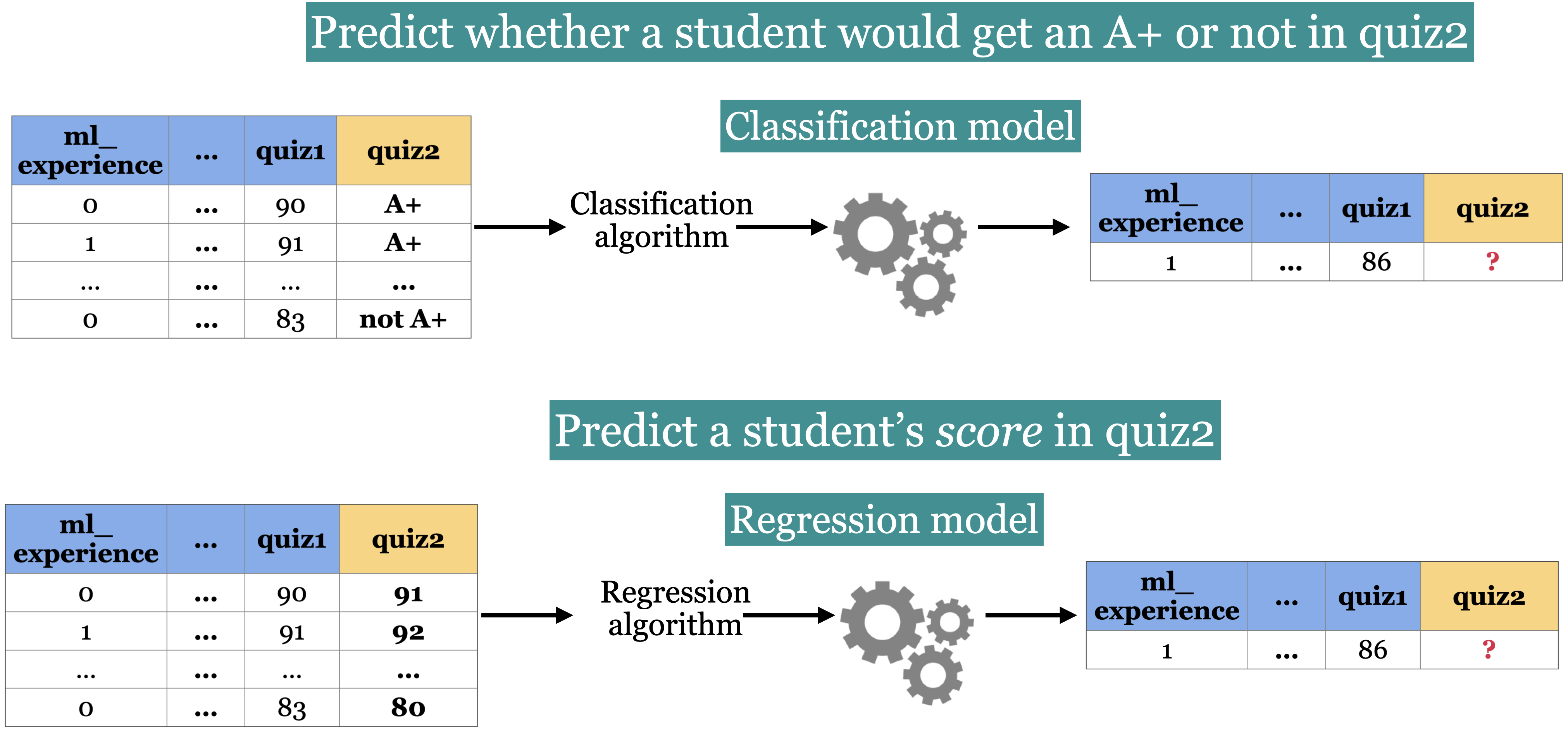
distinguish classification from regression and supervised from unsupervised learning;
build a baseline and explain why it is an essential reference point;
use the scikit-learn fit–predict–score pattern while recognizing that score is model-dependent;
explain at a high level how a decision tree learns rules and makes predictions;
distinguish model parameters from hyperparameters; and
interpret tree depth and decision boundaries as representations of model complexity.

Imports

import os
import sys

import matplotlib.pyplot as plt
import numpy as np
import pandas as pd

sys.path.append(os.path.abspath("code"))

import mglearn
from IPython.display import HTML, display
from plotting_functions import *
from sklearn.dummy import DummyClassifier
from sklearn.tree import DecisionTreeClassifier, DecisionTreeRegressor
from utils import *

plt.rcParams["font.size"] = 16
pd.set_option("display.max_colwidth", 200)

%matplotlib inline

DATA_DIR = "data/"

From a dataset to a first model

Machine learning uses a large vocabulary for a small number of recurring ideas. We will introduce that vocabulary through one running example, establish a simple baseline, and then train our first learned model: a decision tree.

See also

An accompanying video introduces the terminology used in this section.

Representing a supervised learning problem

A supervised learning problem begins with examples for which the outcome is already known. We represent the available information as features and the outcome we want to predict as a target. A learning algorithm uses these examples to construct a model that can make predictions for new cases.

Running example: quiz-grade prediction

For our first model, imagine that students want to anticipate whether they will receive an A+ on Quiz 2. They collect data from a previous offering containing attendance, lab grades, Quiz 1 performance, and the eventual Quiz 2 result. Before looking at the data, pause and identify which quantity is the target, which attributes could be features, and which of those features would actually be available before Quiz 2.

We will use three small datasets in this and the next chapter:

These deliberately small datasets let us inspect every step. Later chapters use larger, messier datasets.

Note

Supporting plotting functions live in book/code/ so that the chapter can focus on the modeling ideas. The code remains available for inspection and reuse.

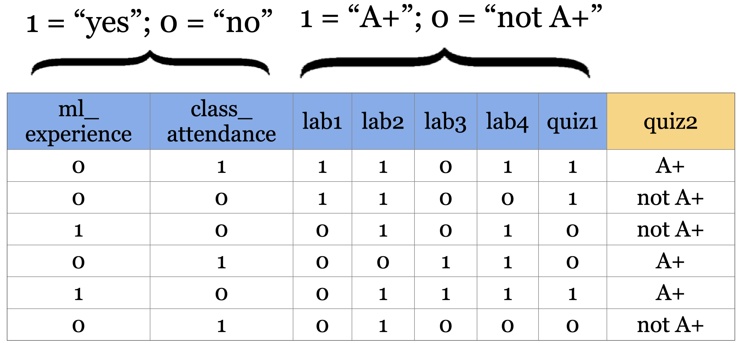
The classification version asks whether a student will receive an A+ rather than predicting the exact grade. Each row describes one student from a previous offering.

classification_df = pd.read_csv(DATA_DIR + "quiz2-grade-toy-classification.csv")
print(classification_df.shape)
classification_df.head()

(21, 8)

	ml_experience	class_attendance	lab1	lab2	lab3	lab4	quiz1	quiz2
0	1	1	92	93	84	91	92	A+
1	1	0	94	90	80	83	91	not A+
2	0	0	78	85	83	80	80	not A+
3	0	1	91	94	92	91	89	A+
4	0	1	77	83	90	92	85	A+

Rows, features, and targets

Supervised-learning data is often organized as a table. Rows are examples, input columns are features, and the column we want to predict is the target.

Feature: An input characteristic available to the model. The feature table is conventionally denoted by \(X\), and the number of features by \(d\).
Target: The outcome we want to predict, conventionally denoted by \(y\).
Example: One observation, represented by a row of feature values. The number of examples is conventionally denoted by \(n\).
Training: The process through which a learning algorithm uses \(X\) and \(y\) to determine a model’s parameters. Training is also called fitting.

Separating the feature table and target

classification_df = pd.read_csv(DATA_DIR + "quiz2-grade-toy-classification.csv")
classification_df.head()

	ml_experience	class_attendance	lab1	lab2	lab3	lab4	quiz1	quiz2
0	1	1	92	93	84	91	92	A+
1	1	0	94	90	80	83	91	not A+
2	0	0	78	85	83	80	80	not A+
3	0	1	91	94	92	91	89	A+
4	0	1	77	83	90	92	85	A+

Before fitting a supervised model, we separate the feature table X from the target vector y. Keeping this distinction explicit helps prevent the answer from accidentally becoming an input to the model.

X = classification_df.drop(columns=["quiz2"])
y = classification_df["quiz2"]
X.head()

	ml_experience	class_attendance	lab1	lab2	lab3	lab4	quiz1
0	1	1	92	93	84	91	92
1	1	0	94	90	80	83	91
2	0	0	78	85	83	80	80
3	0	1	91	94	92	91	89
4	0	1	77	83	90	92	85

y.head()

0        A+
1    not A+
2    not A+
3        A+
4        A+
Name: quiz2, dtype: str

A second example: housing-price prediction

The same representation applies when the target is numerical. Here, each row represents a house, the property attributes form X, and price is y.

housing_df = pd.read_csv(DATA_DIR + "kc_house_data.csv")
housing_df.drop(["id", "date"], axis=1, inplace=True)
HTML(housing_df.head().to_html(index=False))

price	bedrooms	bathrooms	sqft_living	sqft_lot	floors	condition	grade	sqft_above	sqft_basement	yr_built	yr_renovated	zipcode	lat	long	sqft_living15	sqft_lot15
221900.0	3	1.00	1180	5650	1.0	3	7	1180	0	1955	0	98178	47.5112	-122.257	1340	5650
538000.0	3	2.25	2570	7242	2.0	3	7	2170	400	1951	1991	98125	47.7210	-122.319	1690	7639
180000.0	2	1.00	770	10000	1.0	3	6	770	0	1933	0	98028	47.7379	-122.233	2720	8062
604000.0	4	3.00	1960	5000	1.0	5	7	1050	910	1965	0	98136	47.5208	-122.393	1360	5000
510000.0	3	2.00	1680	8080	1.0	3	8	1680	0	1987	0	98074	47.6168	-122.045	1800	7503

X = housing_df.drop(columns=["price"])
y = housing_df["price"]
X.head()

	bedrooms	bathrooms	sqft_living	sqft_lot	floors	condition	grade	sqft_above	sqft_basement	yr_built	yr_renovated	zipcode	lat	long	sqft_living15	sqft_lot15
0	3	1.00	1180	5650	1.0	3	7	1180	0	1955	0	98178	47.5112	-122.257	1340	5650
1	3	2.25	2570	7242	2.0	3	7	2170	400	1951	1991	98125	47.7210	-122.319	1690	7639
2	2	1.00	770	10000	1.0	3	6	770	0	1933	0	98028	47.7379	-122.233	2720	8062
3	4	3.00	1960	5000	1.0	5	7	1050	910	1965	0	98136	47.5208	-122.393	1360	5000
4	3	2.00	1680	8080	1.0	3	8	1680	0	1987	0	98074	47.6168	-122.045	1800	7503

y.head()

0    221900.0
1    538000.0
2    180000.0
3    604000.0
4    510000.0
Name: price, dtype: float64

X.shape

(21613, 18)

Important

Column names are meaningful to people, but most estimators operate on the feature values. A descriptive name does not make a feature informative, and an ambiguous name does not prevent its values from influencing a model.

A compact terminology guide

Different communities often use different words for the same role:

examples = rows = samples = records = instances;
features = inputs = predictors = explanatory variables = covariates;
targets = outputs = outcomes = responses; categorical targets are often called labels; and
training = learning = fitting.

The surrounding context determines which meaning is intended.

See also

The MDS terminology guide provides a broader cross-disciplinary glossary.

Supervised and unsupervised learning

In supervised learning, the training data contains features \(X\) and corresponding targets \(y\). The goal is to learn a mapping that predicts the target for new examples.

In unsupervised learning, the observations have no designated target. The goal may instead be to find groups, discover structure, or construct a concise representation of the data. We return to unsupervised learning later in the book.

Classification and regression

Supervised problems are commonly distinguished by the kind of target:

Classification predicts one of two or more discrete classes—for example, liver disease versus no liver disease, or A+ versus not A+.
Regression predicts a numerical quantity—for example, a house price or percentage grade.

The distinction affects which estimators and evaluation measures are appropriate.

# quiz2 classification toy data
classification_df = pd.read_csv(DATA_DIR + "quiz2-grade-toy-classification.csv")
classification_df.head(4)

	ml_experience	class_attendance	lab1	lab2	lab3	lab4	quiz1	quiz2
0	1	1	92	93	84	91	92	A+
1	1	0	94	90	80	83	91	not A+
2	0	0	78	85	83	80	80	not A+
3	0	1	91	94	92	91	89	A+

# quiz2 regression toy data
regression_df = pd.read_csv(DATA_DIR + "quiz2-grade-toy-regression.csv")
regression_df.head(4)

	ml_experience	class_attendance	lab1	lab2	lab3	lab4	quiz1	quiz2
0	1	1	92	93	84	91	92	90
1	1	0	94	90	80	83	91	84
2	0	0	78	85	83	80	80	82
3	0	1	91	94	92	91	89	92

classification_df

	ml_experience	class_attendance	lab1	lab2	lab3	lab4	quiz1	quiz2
0	1	1	92	93	84	91	92	A+
1	1	0	94	90	80	83	91	not A+
2	0	0	78	85	83	80	80	not A+
3	0	1	91	94	92	91	89	A+
4	0	1	77	83	90	92	85	A+
5	1	0	70	73	68	74	71	not A+
6	1	0	80	88	89	88	91	A+
7	0	1	95	93	69	79	75	not A+
8	0	0	97	90	94	99	80	not A+
9	1	1	95	95	94	94	85	not A+
10	0	1	98	86	95	95	78	A+
11	1	1	95	88	93	92	85	A+
12	1	1	98	96	96	99	100	A+
13	0	1	95	94	96	95	100	A+
14	0	1	95	90	93	95	70	not A+
15	1	0	92	85	67	94	92	not A+
16	0	0	75	91	93	86	85	A+
17	1	0	86	89	65	86	87	not A+
18	1	1	91	93	90	88	82	not A+
19	0	1	77	94	87	81	89	not A+
20	1	1	96	92	92	96	87	A+

classification_df.shape

(21, 8)

Prediction and statistical inference

Prediction asks what outcome a model should assign to a new example. Statistical inference asks what the observed data supports us in concluding about relationships, effects, or populations. For example, predicting recovery time is different from estimating whether a treatment causes recovery to happen sooner.

The goals can complement one another, but strong predictive performance does not by itself establish a causal explanation. In deployed machine-learning systems, the word inference is also sometimes used for the act of generating predictions with an already-fitted model; that operational usage is distinct from statistical inference.

Exercise 2.1: Is machine learning suitable?

Select all problems for which machine learning could be a suitable component. Be prepared to state what examples the system could learn from and where human judgment or explicit rules should remain involved.

1. Identifying objects in digital images.
1. Determining eligibility for a service governed by complete, stable, and explicit rules.
1. Flagging unusual transaction patterns for fraud investigation.
1. Flagging possible abnormalities in medical images for expert review.
1. Providing empathetic support for a person experiencing a mental-health crisis.

Solution

A, C, and D have learnable patterns and plausible sources of labeled examples. B is naturally rule-based when the rules are complete and stable. E requires context, empathy, and accountability that should not be delegated to a predictive model, although carefully scoped tools might support a qualified human.

Exercise 2.2: Supervised or unsupervised?

Select all examples of supervised learning.

1. Finding groups of similar properties in a real-estate dataset.
1. Predicting heart-attack risk from demographic, dietary, and clinical measurements.
1. Grouping news articles by topic.
1. Detecting credit-card fraud from labeled fraudulent and non-fraudulent transactions.
1. Using measured employee performance to investigate which recorded factors predict it.

Solution

B, D, and E are supervised because each requires an observed target. E emphasizes interpretation, so predictive associations should not automatically be treated as causal effects.

Exercise 2.3: Classification or regression?

Select all regression problems.

1. Predicting the price of a house.
1. Predicting whether a house will sell.
1. Predicting a student’s percentage grade.
1. Predicting whether to bicycle tomorrow.
1. Predicting an appropriate numerical thermostat setting.

Solution

A, C, and E have numerical targets and are therefore regression problems.

Exercise 2.4: Define the representation

For each problem below, identify one possible unit of analysis, a target, and several features that would be available at prediction time:

sentiment analysis;
fraud detection; and
face recognition.

Are any of the proposed features ethically sensitive, unavailable at prediction time, or likely to encode the target indirectly?

Establishing a baseline

See also

An accompanying video develops the baseline example in this section.

We are now ready to build a simple supervised model for the quiz-grade problem. Before trying a sophisticated method, we need a reference point that tells us what performance can be achieved with almost no learning.

classification_df = pd.read_csv(DATA_DIR + "quiz2-grade-toy-classification.csv")
classification_df.head()

	ml_experience	class_attendance	lab1	lab2	lab3	lab4	quiz1	quiz2
0	1	1	92	93	84	91	92	A+
1	1	0	94	90	80	83	91	not A+
2	0	0	78	85	83	80	80	not A+
3	0	1	91	94	92	91	89	A+
4	0	1	77	83	90	92	85	A+

classification_df["quiz2"].value_counts()

quiz2
not A+    11
A+        10
Name: count, dtype: int64

The label “not A+” is more common. A strategy that always predicts this majority class ignores every feature, but it may still achieve substantial accuracy. That makes it a useful sanity check.

Why start with a baseline?

Baseline: A simple reference strategy against which more elaborate models can be compared.

For classification, a common baseline always predicts the most frequent training label. A useful learned model should improve on an appropriate baseline in a way that matters for the problem.

A classification baseline with `DummyClassifier`

scikit-learn provides DummyClassifier for simple classification baselines. We will fit a most-frequent baseline to the quiz-grade data.

The `scikit-learn` model-building pattern

Most estimators follow the same interface:

construct the feature table X and target y;
create an estimator;
call fit(X, y) to learn from the training data;
call predict(X_new) to predict new examples; and
evaluate predictions with an appropriate measure.

Reading the data

classification_df.head()

	ml_experience	class_attendance	lab1	lab2	lab3	lab4	quiz1	quiz2
0	1	1	92	93	84	91	92	A+
1	1	0	94	90	80	83	91	not A+
2	0	0	78	85	83	80	80	not A+
3	0	1	91	94	92	91	89	A+
4	0	1	77	83	90	92	85	A+

Create \(X\) and \(y\)

\(X\) → Feature vectors
\(y\) → Target

X = classification_df.drop(columns=["quiz2"])
y = classification_df["quiz2"]

Create a classifier object

import the appropriate classifier
Create an object of the classifier

from sklearn.dummy import DummyClassifier  # import the classifier

dummy_clf = DummyClassifier(strategy="most_frequent")  # Create a classifier object

`fit` the classifier

The “learning” is carried out when we call fit on the classifier object.

dummy_clf.fit(X, y)
# fit the classifier

DummyClassifier(strategy='most_frequent')

In a Jupyter environment, please rerun this cell to show the HTML representation or trust the notebook.
On GitHub, the HTML representation is unable to render, please try loading this page with nbviewer.org.

DummyClassifier

?Documentation for DummyClassifieriFitted

Parameters

	strategy strategy: {"most_frequent", "prior", "stratified", "uniform", "constant"}, default="prior" Strategy to use to generate predictions. * "most_frequent": the `predict` method always returns the most frequent class label in the observed `y` argument passed to `fit`. The `predict_proba` method returns the matching one-hot encoded vector. * "prior": the `predict` method always returns the most frequent class label in the observed `y` argument passed to `fit` (like "most_frequent"). ``predict_proba`` always returns the empirical class distribution of `y` also known as the empirical class prior distribution. * "stratified": the `predict_proba` method randomly samples one-hot vectors from a multinomial distribution parametrized by the empirical class prior probabilities. The `predict` method returns the class label which got probability one in the one-hot vector of `predict_proba`. Each sampled row of both methods is therefore independent and identically distributed. * "uniform": generates predictions uniformly at random from the list of unique classes observed in `y`, i.e. each class has equal probability. * "constant": always predicts a constant label that is provided by the user. This is useful for metrics that evaluate a non-majority class. .. versionchanged:: 0.24 The default value of `strategy` has changed to "prior" in version 0.24.	'most_frequent'
	random_state random_state: int, RandomState instance or None, default=None Controls the randomness to generate the predictions when ``strategy='stratified'`` or ``strategy='uniform'``. Pass an int for reproducible output across multiple function calls. See :term:`Glossary <random_state>`.	None
	constant constant: int or str or array-like of shape (n_outputs,), default=None The explicit constant as predicted by the "constant" strategy. This parameter is useful only for the "constant" strategy.	None

Fitted attributes

Name	Type	Value
class_prior_ class_prior_: ndarray of shape (n_classes,) or list of such arrays Frequency of each class observed in `y`. For multioutput classification problems, this is computed independently for each output.	ndarray[float64](2,)	[0.48,0.52]
classes_ classes_: ndarray of shape (n_classes,) or list of such arrays Unique class labels observed in `y`. For multi-output classification problems, this attribute is a list of arrays as each output has an independent set of possible classes.	ndarray[object](2,)	['A+','not A+']
feature_names_in_ feature_names_in_: ndarray of shape (`n_features_in_`,) Names of features seen during :term:`fit`. Defined only when `X` has feature names that are all strings.	ndarray[object](7,)	['ml_experience','class_attendance','lab1',...,'lab3','lab4','quiz1']
n_classes_ n_classes_: int or list of int Number of label for each output.	int	2
n_features_in_ n_features_in_: int Number of features seen during :term:`fit`.	int	7
n_outputs_ n_outputs_: int Number of outputs.	int	1
sparse_output_ sparse_output_: bool True if the array returned from predict is to be in sparse CSC format. Is automatically set to True if the input `y` is passed in sparse format.	bool	False

`predict` the target of given examples

We can predict the target of examples by calling predict on the classifier object.

dummy_clf.predict(X)  # predict using the trained classifier

array(['not A+', 'not A+', 'not A+', 'not A+', 'not A+', 'not A+',
       'not A+', 'not A+', 'not A+', 'not A+', 'not A+', 'not A+',
       'not A+', 'not A+', 'not A+', 'not A+', 'not A+', 'not A+',
       'not A+', 'not A+', 'not A+'], dtype='<U6')

Evaluating with `score`

An estimator’s score method provides a convenient default measure, but its meaning depends on the estimator. For classifiers it is usually accuracy—the proportion of correctly predicted targets:

\[ ext{accuracy} = rac{ ext{correct predictions}}{ ext{total predictions}}. \]

Always check what score returns before interpreting it as model quality.

print("The accuracy of the model on the training data: %0.3f" % (dummy_clf.score(X, y)))

The accuracy of the model on the training data: 0.524

Classification error is often defined as \(1 - ext{accuracy}\). Calling a classifier’s score(X, y) typically runs predict(X), compares the predictions with y, and returns accuracy.

For now we evaluate on the same small dataset used for fitting. This demonstrates the API, but it does not tell us how well the model will work on new data. Chapter 3 addresses that central problem.

print(
    "The error of the model on the training data: %0.3f" % (1 - dummy_clf.score(X, y))
)

The error of the model on the training data: 0.476

The `fit`, `predict`, and `score` pattern

The complete baseline workflow is shown below.

# Create `X` and `y` from the given data
X = classification_df.drop(columns=["quiz2"])
y = classification_df["quiz2"]

clf = DummyClassifier(strategy="most_frequent")  # Create a class object
clf.fit(X, y)  # Train/fit the model
print(clf.score(X, y))  # Assess the model

new_examples = [[0, 1, 92, 90, 95, 93, 92], [1, 1, 92, 93, 94, 92]]
clf.predict(new_examples)  # Predict on some new data using the trained model

0.5238095238095238

array(['not A+', 'not A+'], dtype='<U6')

Note

You will investigate classification baselines more fully in the exercises and lab.

A regression baseline with `DummyRegressor`

For regression, DummyRegressor can predict a constant such as the training-set mean or median. Its default score is \(R^2\), not accuracy.

The code below applies the same fit and predict pattern to the numerical version of the quiz-grade problem.

from sklearn.dummy import DummyRegressor

regression_df = pd.read_csv(DATA_DIR + "quiz2-grade-toy-regression.csv")  # Read data
X = regression_df.drop(columns=["quiz2"])  # Create `X` and `y` from the given data
y = regression_df["quiz2"]
reg = DummyRegressor()  # Create a class object
reg.fit(X, y)  # Train/fit the model
reg.score(X, y)  # Assess the model
new_examples = [[0, 1, 92, 90, 95, 93, 92], [1, 1, 92, 93, 94, 92]]
reg.predict(new_examples)  # Predict on some new data using the trained model

array([86.28571429, 86.28571429])

fit and predict play the same roles for regression and classification, but the default score differs. For regressors, score normally returns \(R^2\):

\(R^2=1\) represents perfect predictions;
a mean-prediction baseline usually has \(R^2=0\) on the data used to evaluate that mean; and
\(R^2<0\) means the predictions are worse than predicting that mean.

We study regression evaluation measures in detail later in the book.

reg.score(X, y)

0.0

Exercise 2.5: Order the modeling steps

Put the following steps in a sensible order:

call score with labeled evaluation data;
call predict on new examples;
create an estimator;
construct X and y; and
call fit.

Learning rules with decision trees

See also

An accompanying video introduces decision trees.

From hand-written rules to learned rules

Can we do better than the majority-class baseline? One option is to write nested if/else rules using attendance and previous grades. To make the idea easy to visualize, first imagine that the feature values have been converted to binary indicators.

Look for combinations that distinguish A+ from not A+. A hand-written program might begin like this:

if class_attendance == 1 and quiz1 == 1:
    prediction = "A+"
elif class_attendance == 1 and lab3 == 1 and lab4 == 1:
    prediction = "A+"
else:
    prediction = "not A+"

Even with seven binary features, the number of possible combinations becomes difficult to manage.

A decision tree learns a hierarchy of these questions from examples rather than requiring us to enumerate the rules by hand. Before fitting one, inspect the examples above: which single yes/no question seems most effective at separating A+ from not A+? A useful question creates groups whose outcomes are more homogeneous than the original group.

The decision-tree idea

A decision tree resembles the Twenty Questions game. At each node it asks a question about one feature and follows a branch based on the answer. Training determines which questions to ask; prediction follows the learned path to an answer.

Building decision trees with `sklearn`

Let’s binarize our toy dataset for simplicity.

classification_df = pd.read_csv(DATA_DIR + "quiz2-grade-toy-classification.csv")
X = classification_df.drop(columns=["quiz2"])
y = classification_df["quiz2"]

X_binary = X.copy()
columns = ["lab1", "lab2", "lab3", "lab4", "quiz1"]
for col in columns:
    X_binary[col] = X_binary[col].apply(lambda x: 1 if x >= 90 else 0)
X_binary.head()

	ml_experience	class_attendance	lab1	lab2	lab3	lab4	quiz1
0	1	1	1	1	0	1	1
1	1	0	1	1	0	0	1
2	0	0	0	0	0	0	0
3	0	1	1	1	1	1	0
4	0	1	0	0	1	1	0

y.head()

0        A+
1    not A+
2    not A+
3        A+
4        A+
Name: quiz2, dtype: str

`DummyClassifier` on quiz2 grade prediction toy dataset

dummy_clf = DummyClassifier(strategy="most_frequent")
dummy_clf.fit(X_binary, y)
dummy_clf.score(X_binary, y)

0.5238095238095238

`DecisionTreeClassifier` on quiz2 grade prediction toy dataset

from sklearn.tree import DecisionTreeClassifier

model = DecisionTreeClassifier()  # Create a decision tree
model.fit(X_binary, y)  # Fit a decision tree
model.score(X_binary, y)  # Assess the model

0.9047619047619048

The decision tree has much higher training accuracy than the dummy baseline. That is encouraging, but it does not yet establish that the tree will predict new students well. We will return to this distinction at the end of the chapter.

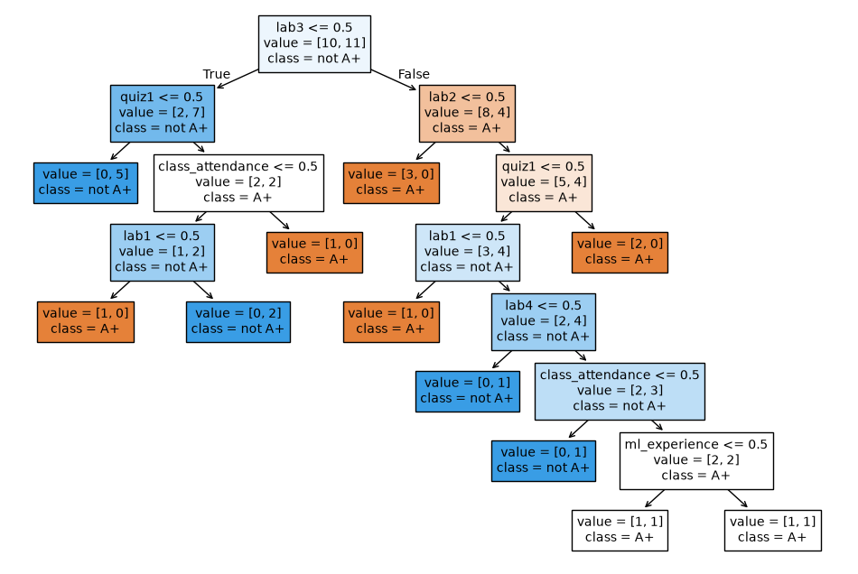
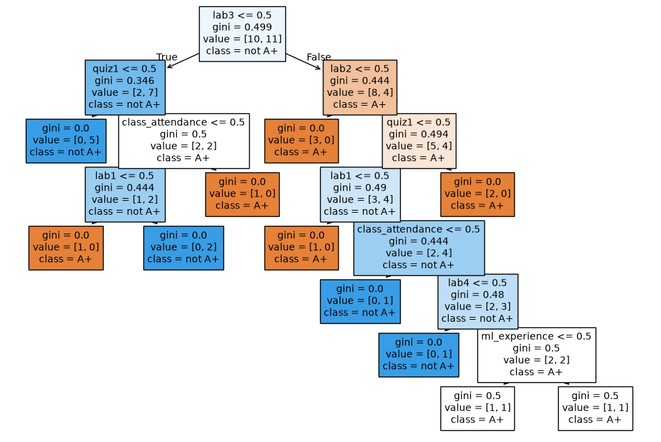
# Call the custom_plot_tree function to visualize the customized tree
width = 12
height = 8
plt.figure(figsize=(width, height))
custom_plot_tree(
    model,
    feature_names=X_binary.columns.tolist(),
    class_names=["A+", "not A+"],
    impurity=False,
    fontsize=10,
)

Reading a decision tree

Root node: The first question asked by the tree.
Branch: A connection representing the result of a question.
Internal node: A subsequent question within the tree.
Leaf node: The prediction produced after following a path through the tree.
Tree depth: The number of edges on the longest path from the root to a leaf.

How does prediction work?

new_example = np.array([[0, 1, 0, 0, 1, 1, 1]])
pd.DataFrame(data=new_example, columns=X.columns)

	ml_experience	class_attendance	lab1	lab2	lab3	lab4	quiz1
0	0	1	0	0	1	1	1

plt.figure(figsize=(width, height))
custom_plot_tree(
    model,
    feature_names=X_binary.columns.tolist(),
    class_names=["A+", "not A+"],
    impurity=False,
    fontsize=10,
)

What’s the prediction for the new example?

model.predict(new_example)

/Users/kvarada/CS/2026-27/cpsc330-book/.venv/lib/python3.12/site-packages/sklearn/utils/validation.py:2827: UserWarning: X does not have valid feature names, but DecisionTreeClassifier was fitted with feature names
  warnings.warn(

array(['A+'], dtype=object)

To predict for a new example, begin at the root, answer the question at each node, and follow the corresponding branch. The leaf at the end of the path supplies the prediction. Features that do not appear along that path do not affect that prediction.

How does fitting work conceptually?

During fitting, the algorithm searches over many possible feature-and-threshold questions and possible orders in which to ask them. It prefers questions that divide the training examples into increasingly homogeneous groups. The selected questions and thresholds become model parameters.

Choosing splits

At each node, a classification tree compares candidate questions using a measure of class impurity. Common criteria include the Gini index and entropy. A question is useful when the resulting groups contain more certain, homogeneous outcomes. The exact search and optimization details are beyond this course, but the result is a hierarchy of data-derived rules.

from sklearn.tree import DecisionTreeClassifier

model = DecisionTreeClassifier()  # Create a decision tree
model.fit(X_binary, y)  # Fit a decision tree
plt.figure(figsize=(width, height))
custom_plot_tree(
    model,
    feature_names=X_binary.columns.tolist(),
    class_names=["A+", "not A+"],
    fontsize=10,
)

Note

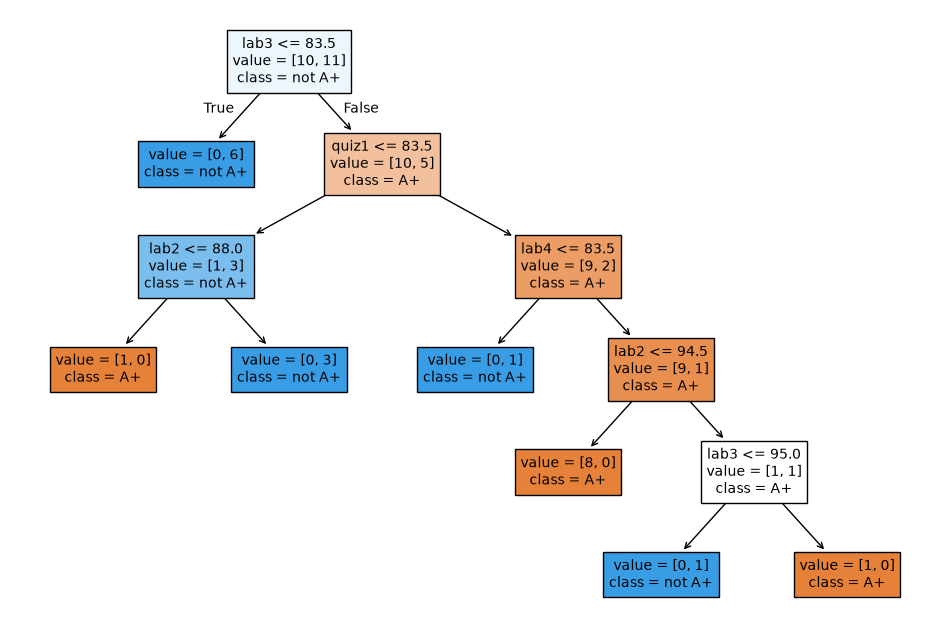
Decision trees can split both categorical representations and numerical features. For a numerical feature, fitting also learns a threshold—for example, quiz1 <= 88.5.

Trees with numerical features

X.head()

	ml_experience	class_attendance	lab1	lab2	lab3	lab4	quiz1
0	1	1	92	93	84	91	92
1	1	0	94	90	80	83	91
2	0	0	78	85	83	80	80
3	0	1	91	94	92	91	89
4	0	1	77	83	90	92	85

model = DecisionTreeClassifier()
model.fit(X, y)
plt.figure(figsize=(width, height))
custom_plot_tree(
    model,
    feature_names=X_binary.columns.tolist(),
    class_names=["A+", "not A+"],
    impurity=False,
    fontsize=10,
)

Decision trees for regression

Decision trees can also predict numerical targets. A DecisionTreeRegressor uses the same fit and predict interface, but chooses splits using a regression criterion such as squared error. Its default score is \(R^2\), which can be negative when predictions are worse than the mean baseline.

regression_df = pd.read_csv(DATA_DIR + "quiz2-grade-toy-regression.csv")
regression_df.head()

	ml_experience	class_attendance	lab1	lab2	lab3	lab4	quiz1	quiz2
0	1	1	92	93	84	91	92	90
1	1	0	94	90	80	83	91	84
2	0	0	78	85	83	80	80	82
3	0	1	91	94	92	91	89	92
4	0	1	77	83	90	92	85	90

X = regression_df.drop(["quiz2"], axis=1)
y = regression_df["quiz2"]

depth = 2
reg_model = DecisionTreeRegressor(max_depth=depth)
reg_model.fit(X, y)
regression_df["predicted_quiz2"] = reg_model.predict(X)
print("R^2 score on the training data: %0.3f\n\n" % (reg_model.score(X, y)))
regression_df.head()

R^2 score on the training data: 0.989

	ml_experience	class_attendance	lab1	lab2	lab3	lab4	quiz1	quiz2	predicted_quiz2
0	1	1	92	93	84	91	92	90	90.333333
1	1	0	94	90	80	83	91	84	83.000000
2	0	0	78	85	83	80	80	82	83.000000
3	0	1	91	94	92	91	89	92	92.000000
4	0	1	77	83	90	92	85	90	90.333333

Exercise 2.6: Baselines and decision trees

Select all true statements.

1. Changing the feature representation necessarily changes a most-frequent DummyClassifier prediction.
1. predict receives X, whereas fit and score receive both X and y.
1. Decision-tree features must be binary.
1. A decision tree predicts by routing an example from the root to a leaf.

Solution

B and D are true. A most-frequent baseline ignores X, and decision trees can split numerical features by learning thresholds.

Model controls and decision boundaries

We now separate what a tree learns from the choices that control how it learns, then visualize how those choices affect its predictions.

See also

An accompanying video discusses parameters, hyperparameters, and decision boundaries.

Parameters

Fitting a decision tree determines which feature to inspect and which threshold to use at each node. These learned values are the model’s parameters. They are stored by the fitted estimator and used during prediction.

classification_df = pd.read_csv(DATA_DIR + "quiz2-grade-toy-classification.csv")
X = classification_df.drop(columns=["quiz2"])
y = classification_df["quiz2"]
model = DecisionTreeClassifier()
model.fit(X, y);

plt.figure(figsize=(width, height))
custom_plot_tree(
    model,
    feature_names=X_binary.columns.tolist(),
    class_names=["A+", "not A+"],
    impurity=False,
    fontsize=10,
)

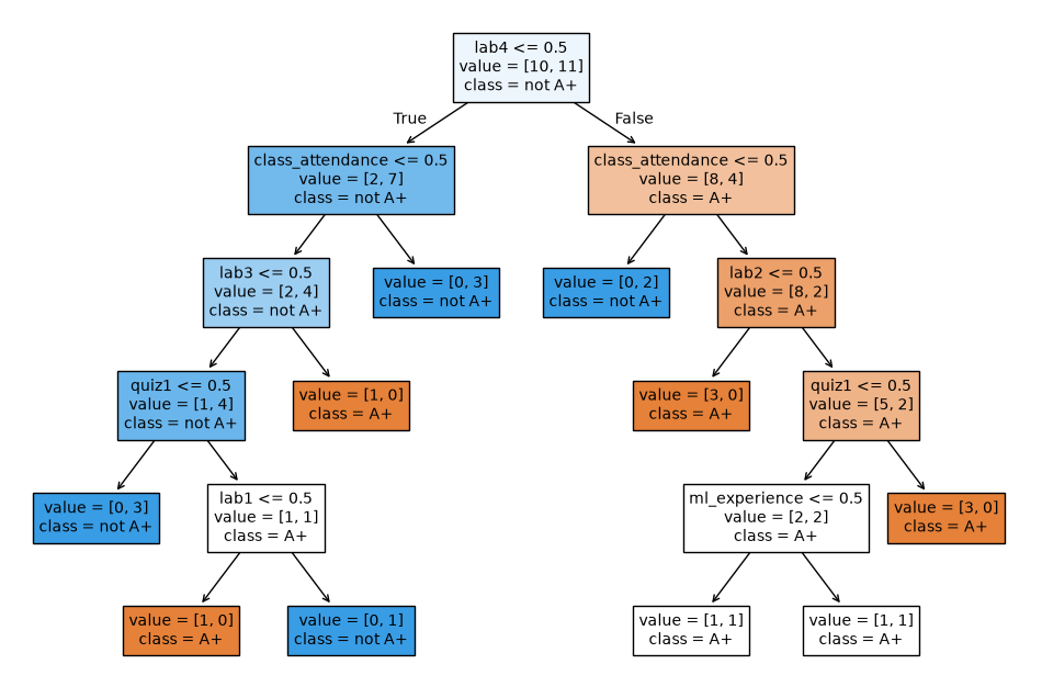
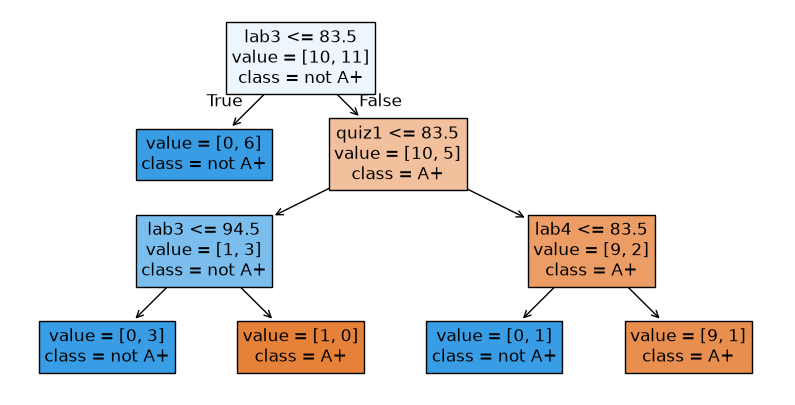
With the default settings, a decision tree can continue splitting until its leaves are pure or another stopping condition is reached.

A very deep tree may create rules that describe only one or two training examples. We can control this behavior with hyperparameters such as the maximum tree depth.

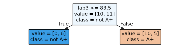
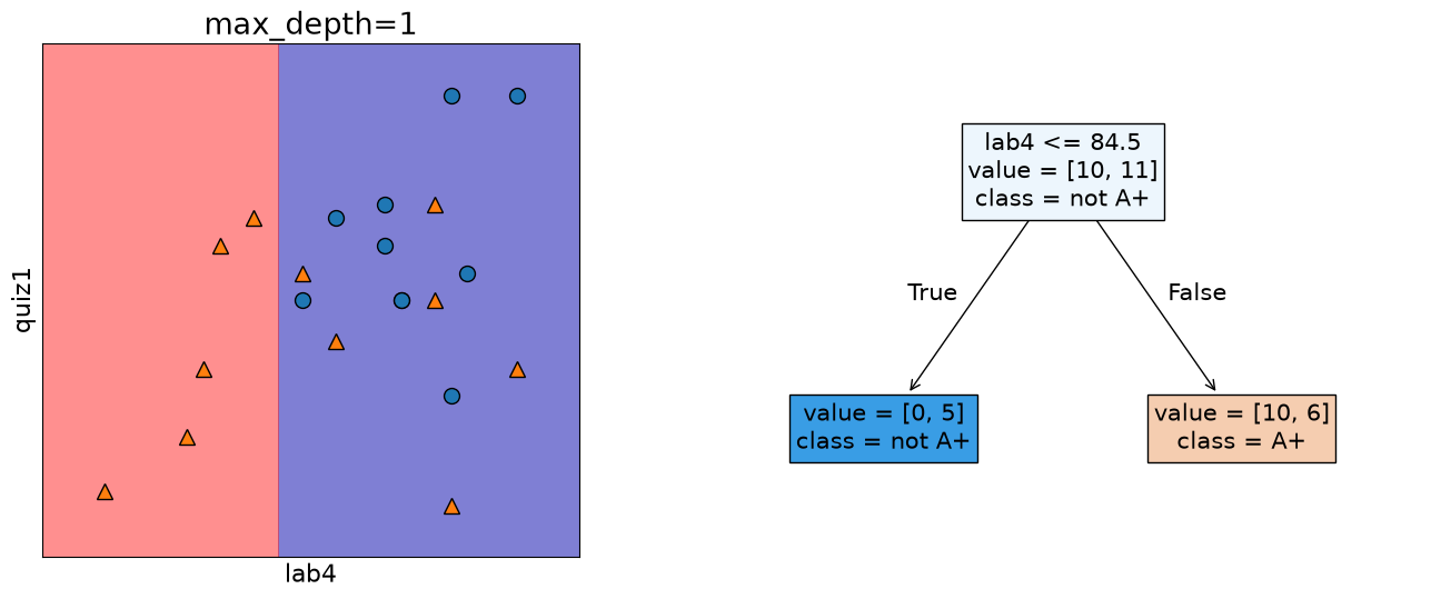
A decision stump: `max_depth=1`

A tree with one split is called a decision stump.

model = DecisionTreeClassifier(max_depth=1)
model.fit(X, y)
width = 8
height = 2
plt.figure(figsize=(width, height))
custom_plot_tree(
    model,
    feature_names=X_binary.columns.tolist(),
    class_names=["A+", "not A+"],
    impurity=False,
    fontsize=12,
)  # custom function defined in code/utils.py

max_depth is a hyperparameter: a setting chosen before fitting that controls which trees the algorithm is allowed to learn.

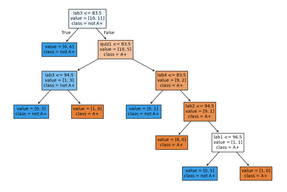
A deeper tree: `max_depth=3`

model = DecisionTreeClassifier(
    max_depth=3
)  # Let's try another value for the hyperparameter
model.fit(X, y)
width = 10
height = 5
plt.figure(figsize=(width, height))

custom_plot_tree(
    model,
    feature_names=X_binary.columns.tolist(),
    class_names=["A+", "not A+"],
    impurity=False,
    fontsize=12,
)

Parameters and hyperparameters

Parameters: Values learned from data during fit, such as split features and thresholds. The fitted model needs them to make predictions.
Hyperparameters: Settings chosen before fit that control the learning process or model family. They may be selected using domain knowledge, heuristics, or a systematic validation procedure.

Important

In scikit-learn, hyperparameters are normally supplied when an estimator is constructed. Fitted parameters are learned later by calling fit.

Besides max_depth, commonly used decision-tree hyperparameters include min_samples_split, min_samples_leaf, and max_leaf_nodes. Each constrains the complexity of the learned tree in a different way.

See also

See the DecisionTreeClassifier documentation for the complete estimator interface and hyperparameters.

Decision boundaries

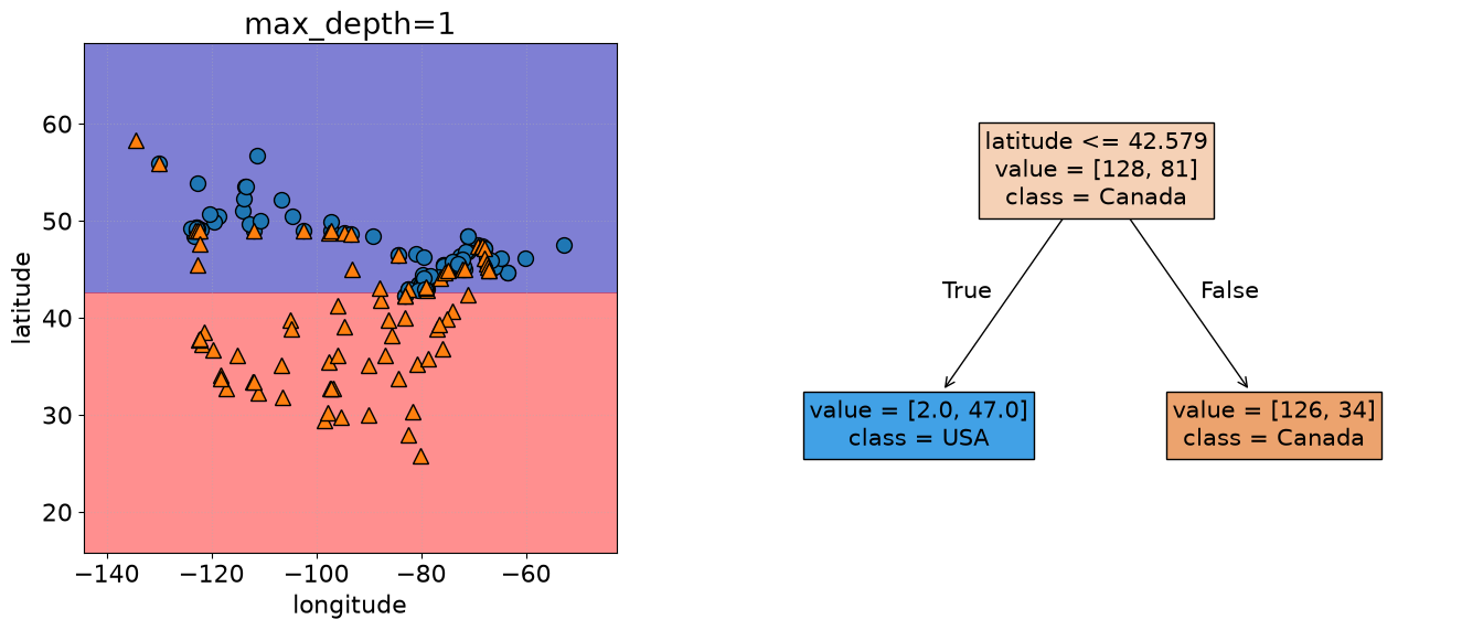
A fitted classifier partitions the possible feature values into regions assigned to different classes. The border between those regions is its decision boundary. With two features, we can draw this boundary and see how model complexity changes it.

Quiz-grade example

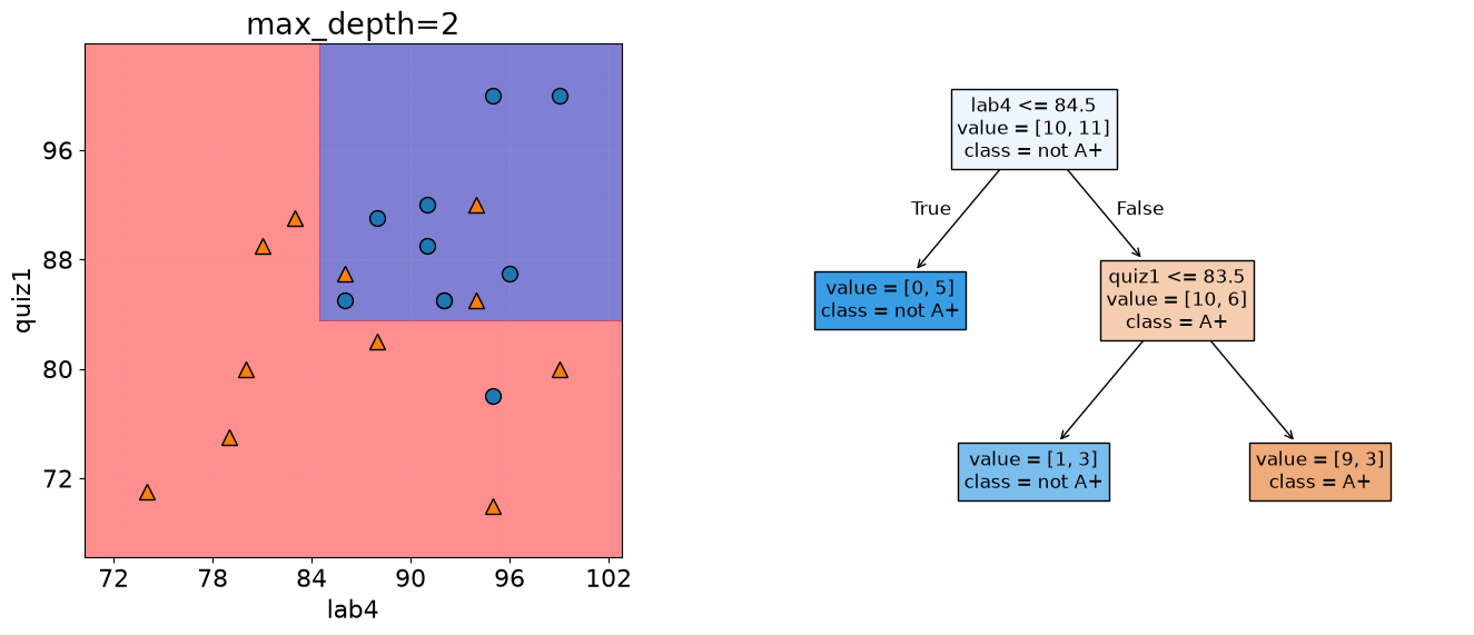
For visualization, we fit trees using only lab4 and quiz1.

X_subset = X[["lab4", "quiz1"]]
X_subset.head()

	lab4	quiz1
0	91	92
1	83	91
2	80	80
3	91	89
4	92	85

Decision boundary with `max_depth=1`

depth = 1  # decision stump
model = DecisionTreeClassifier(max_depth=depth)
model.fit(X_subset.values, y)
plot_tree_decision_boundary_and_tree(
    model, X_subset, y, x_label="lab4", y_label="quiz1", fontsize=15
)

The two colored regions show the classes predicted for possible combinations of lab4 and quiz1. A depth-one tree creates a single horizontal or vertical boundary because it asks one threshold question.

Decision boundary with `max_depth=2`

model = DecisionTreeClassifier(max_depth=2)
model.fit(X_subset.values, y)
plot_tree_decision_boundary_and_tree(
    model, X_subset, y, x_label="lab4", y_label="quiz1", fontsize=12
)

A second level allows the model to divide another region, producing a more detailed decision boundary.

Decision boundary with `max_depth=5`

model = DecisionTreeClassifier(max_depth=5)
model.fit(X_subset.values, y)
plot_tree_decision_boundary_and_tree(
    model, X_subset, y, x_label="lab4", y_label="quiz1", fontsize=8
)

At depth five, the boundary follows the training examples much more closely. Greater detail lowers training error, but whether it improves predictions for new examples remains unresolved.

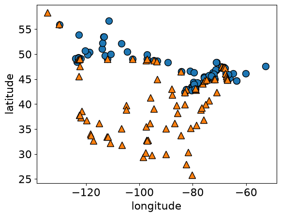
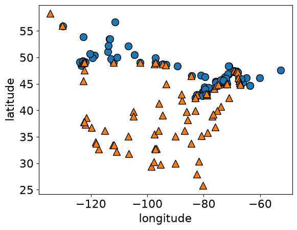
Canada–USA cities example

Suppose we observe the longitude, latitude, and country of several cities near the Canada–USA border. Can a decision tree learn a boundary that predicts the country of a new coordinate?

### US Canada cities data
df = pd.read_csv(DATA_DIR + "canada_usa_cities.csv")
df

	longitude	latitude	country
0	-130.0437	55.9773	USA
1	-134.4197	58.3019	USA
2	-123.0780	48.9854	USA
3	-122.7436	48.9881	USA
4	-122.2691	48.9951	USA
...	...	...	...
204	-72.7218	45.3990	Canada
205	-66.6458	45.9664	Canada
206	-79.2506	42.9931	Canada
207	-72.9406	45.6275	Canada
208	-79.4608	46.3092	Canada

209 rows × 3 columns

X = df[["longitude", "latitude"]]

y = df["country"]

mglearn.discrete_scatter(X.iloc[:, 0], X.iloc[:, 1], y)
plt.xlabel("longitude")
plt.ylabel("latitude");

The geographic boundary

In reality, the Canada–USA boundary is known:

Image source

Our model does not receive this boundary. It approximates one using only the limited labeled examples in the training data.

model = DecisionTreeClassifier(max_depth=1)
model.fit(X.values, y)
plot_tree_decision_boundary_and_tree(
    model,
    X,
    y,
    height=6,
    width=16,
    fontsize=15,
    eps=10,
    x_label="longitude",
    y_label="latitude",
)

model = DecisionTreeClassifier(max_depth=2)
model.fit(X.values, y)
plot_tree_decision_boundary_and_tree(
    model,
    X,
    y,
    height=6,
    width=16,
    fontsize=12,
    eps=10,
    x_label="longitude",
    y_label="latitude",
)

Summary

This chapter established the vocabulary and workflow used throughout the book:

examples are represented by feature rows in \(X\), with targets in \(y\);
classification predicts discrete labels, whereas regression predicts numerical values;
baselines provide reference performance that a useful model should improve upon;
scikit-learn estimators share the fit and predict interface, while score is model-dependent;
decision trees learn hierarchies of feature-threshold questions;
fitted split features and thresholds are parameters, while settings such as max_depth are hyperparameters; and
increasing tree depth creates a more detailed decision boundary and can reduce training error.

The question that remains

A sufficiently deep tree can classify every training example correctly. Does that mean it will predict new examples well? Chapter 3 introduces data splitting, cross-validation, underfitting, and overfitting to answer this question.

From a dataset to a first model

Representing a supervised learning problem

Running example: quiz-grade prediction

Rows, features, and targets

Separating the feature table and target

A second example: housing-price prediction

A compact terminology guide

Supervised and unsupervised learning

Classification and regression

Prediction and statistical inference

Exercise 2.1: Is machine learning suitable?

Exercise 2.2: Supervised or unsupervised?

Exercise 2.3: Classification or regression?

Exercise 2.4: Define the representation

Establishing a baseline

Why start with a baseline?

A classification baseline with DummyClassifier

The scikit-learn model-building pattern

Reading the data

Create \(X\) and \(y\)

Create a classifier object

fit the classifier

predict the target of given examples

Evaluating with score

The fit, predict, and score pattern

A regression baseline with DummyRegressor

Exercise 2.5: Order the modeling steps

Learning rules with decision trees

From hand-written rules to learned rules

The decision-tree idea

Building decision trees with sklearn

DummyClassifier on quiz2 grade prediction toy dataset

DecisionTreeClassifier on quiz2 grade prediction toy dataset

Reading a decision tree

How does prediction work?

How does fitting work conceptually?

Choosing splits

Trees with numerical features

Decision trees for regression

Exercise 2.6: Baselines and decision trees

Model controls and decision boundaries

Parameters

A decision stump: max_depth=1

A deeper tree: max_depth=3

Parameters and hyperparameters

Decision boundaries

Quiz-grade example

Decision boundary with max_depth=1

Decision boundary with max_depth=2

Decision boundary with max_depth=5

Canada–USA cities example

The geographic boundary

Summary

A classification baseline with `DummyClassifier`

The `scikit-learn` model-building pattern

`fit` the classifier

`predict` the target of given examples

Evaluating with `score`

The `fit`, `predict`, and `score` pattern

A regression baseline with `DummyRegressor`

Building decision trees with `sklearn`

`DummyClassifier` on quiz2 grade prediction toy dataset

`DecisionTreeClassifier` on quiz2 grade prediction toy dataset

A decision stump: `max_depth=1`

A deeper tree: `max_depth=3`

Decision boundary with `max_depth=1`

Decision boundary with `max_depth=2`

Decision boundary with `max_depth=5`