Lecture 3 demo: ML fundamentals

Varada Kolhatkar

Lecture 3 Class Demo

from pathlib import Path

import matplotlib.pyplot as plt
import numpy as np
import pandas as pd
from sklearn.dummy import DummyRegressor
from sklearn.model_selection import cross_validate, train_test_split
from sklearn.tree import DecisionTreeRegressor, plot_tree
RANDOM_STATE = 123

Let’s use housing prices to investigate a question from last lecture: does a great training score mean we have a useful model?

We’ll build a first model, question how we evaluated it, and improve our workflow together. The opening steps are deliberately naive: we explore and fit on all the data before introducing splitting. By the end, we’ll explain what we would do differently on a fresh project.

How to use this notebook: pause at the questions before running the next cell. Code cells marked TODO contain the worked solution for now; try describing or writing your approach before reading it. You can hide the solution while we work together.

Run cells in order in JupyterLab or VS Code. Put kc_house_data.csv in a data folder beside this notebook, and use a kernel with NumPy, pandas, Matplotlib, and scikit-learn installed.

Chapter 3: ML fundamentals

The prediction problem

The King County housing dataset contains records of house sales, including sale prices and information about each property. The data are available from House Sales in King County, USA.

Imagine that we want to estimate a property’s sale price from its recorded characteristics.

data_path = Path("data/kc_house_data.csv")

housing_df = pd.read_csv(data_path)
housing_df.head()

	id	date	price	bedrooms	bathrooms	sqft_living	sqft_lot	floors	...	grade	sqft_above	sqft_basement	yr_built	yr_renovated	zipcode	lat	long	sqft_living15	sqft_lot15
0	7129300520	20141013T000000	221900.0	3	1.00	1180	5650	1.0	...	7	1180	0	1955	0	98178	47.5112	-122.257	1340	5650
1	6414100192	20141209T000000	538000.0	3	2.25	2570	7242	2.0	...	7	2170	400	1951	1991	98125	47.7210	-122.319	1690	7639
2	5631500400	20150225T000000	180000.0	2	1.00	770	10000	1.0	...	6	770	0	1933	0	98028	47.7379	-122.233	2720	8062
3	2487200875	20141209T000000	604000.0	4	3.00	1960	5000	1.0	...	7	1050	910	1965	0	98136	47.5208	-122.393	1360	5000
4	1954400510	20150218T000000	510000.0	3	2.00	1680	8080	1.0	...	8	1680	0	1987	0	98074	47.6168	-122.045	1800	7503

5 rows × 21 columns

❓❓ Questions for you

Discuss before coding

What does one example represent? What is the target?
Is this a classification problem or a regression problem?
What would it mean for this model to generalize?

Exploratory Data Analysis (EDA)

Before building anything, let’s get to know these house sales.

TODO: take a first look. How many rows and columns do we have? What do the summaries and missing-value counts tell us?

We’re using the full dataset in this opening demonstration. On a fresh project, we would reserve test data before EDA. Keep track of this shortcut—we’ll return to it at the end.

# How many data points do we have? 
housing_df.shape[0]

# What are the columns in the dataset? 
housing_df.columns

Index(['id', 'date', 'price', 'bedrooms', 'bathrooms', 'sqft_living',
       'sqft_lot', 'floors', 'waterfront', 'view', 'condition', 'grade',
       'sqft_above', 'sqft_basement', 'yr_built', 'yr_renovated', 'zipcode',
       'lat', 'long', 'sqft_living15', 'sqft_lot15'],
      dtype='str')

What ranges do the numerical features have? Let’s try describe() and info().

housing_df.describe()

	id	price	bedrooms	bathrooms	sqft_living	sqft_lot	floors	waterfront	view	condition	grade	sqft_above	sqft_basement	yr_built	yr_renovated	zipcode	lat	long	sqft_living15	sqft_lot15
count	2.161300e+04	2.161300e+04	21613.000000	21613.000000	21613.000000	2.161300e+04	21613.000000	21613.000000	21613.000000	21613.000000	21613.000000	21613.000000	21613.000000	21613.000000	21613.000000	21613.000000	21613.000000	21613.000000	21613.000000	21613.000000
mean	4.580302e+09	5.400881e+05	3.370842	2.114757	2079.899736	1.510697e+04	1.494309	0.007542	0.234303	3.409430	7.656873	1788.390691	291.509045	1971.005136	84.402258	98077.939805	47.560053	-122.213896	1986.552492	12768.455652
std	2.876566e+09	3.671272e+05	0.930062	0.770163	918.440897	4.142051e+04	0.539989	0.086517	0.766318	0.650743	1.175459	828.090978	442.575043	29.373411	401.679240	53.505026	0.138564	0.140828	685.391304	27304.179631
min	1.000102e+06	7.500000e+04	0.000000	0.000000	290.000000	5.200000e+02	1.000000	0.000000	0.000000	1.000000	1.000000	290.000000	0.000000	1900.000000	0.000000	98001.000000	47.155900	-122.519000	399.000000	651.000000
25%	2.123049e+09	3.219500e+05	3.000000	1.750000	1427.000000	5.040000e+03	1.000000	0.000000	0.000000	3.000000	7.000000	1190.000000	0.000000	1951.000000	0.000000	98033.000000	47.471000	-122.328000	1490.000000	5100.000000
50%	3.904930e+09	4.500000e+05	3.000000	2.250000	1910.000000	7.618000e+03	1.500000	0.000000	0.000000	3.000000	7.000000	1560.000000	0.000000	1975.000000	0.000000	98065.000000	47.571800	-122.230000	1840.000000	7620.000000
75%	7.308900e+09	6.450000e+05	4.000000	2.500000	2550.000000	1.068800e+04	2.000000	0.000000	0.000000	4.000000	8.000000	2210.000000	560.000000	1997.000000	0.000000	98118.000000	47.678000	-122.125000	2360.000000	10083.000000
max	9.900000e+09	7.700000e+06	33.000000	8.000000	13540.000000	1.651359e+06	3.500000	1.000000	4.000000	5.000000	13.000000	9410.000000	4820.000000	2015.000000	2015.000000	98199.000000	47.777600	-121.315000	6210.000000	871200.000000

housing_df.info()

<class 'pandas.DataFrame'>
RangeIndex: 21613 entries, 0 to 21612
Data columns (total 21 columns):
 #   Column         Non-Null Count  Dtype  
---  ------         --------------  -----  
 0   id             21613 non-null  int64  
 1   date           21613 non-null  str    
 2   price          21613 non-null  float64
 3   bedrooms       21613 non-null  int64  
 4   bathrooms      21613 non-null  float64
 5   sqft_living    21613 non-null  int64  
 6   sqft_lot       21613 non-null  int64  
 7   floors         21613 non-null  float64
 8   waterfront     21613 non-null  int64  
 9   view           21613 non-null  int64  
 10  condition      21613 non-null  int64  
 11  grade          21613 non-null  int64  
 12  sqft_above     21613 non-null  int64  
 13  sqft_basement  21613 non-null  int64  
 14  yr_built       21613 non-null  int64  
 15  yr_renovated   21613 non-null  int64  
 16  zipcode        21613 non-null  int64  
 17  lat            21613 non-null  float64
 18  long           21613 non-null  float64
 19  sqft_living15  21613 non-null  int64  
 20  sqft_lot15     21613 non-null  int64  
dtypes: float64(5), int64(15), str(1)
memory usage: 3.5 MB

Does a numerical dtype always mean a column should be treated as a numerical measurement?

# TODO: check whether any columns have missing values.
housing_df.isna().sum()

id               0
date             0
price            0
bedrooms         0
bathrooms        0
sqft_living      0
sqft_lot         0
floors           0
waterfront       0
view             0
condition        0
grade            0
sqft_above       0
sqft_basement    0
yr_built         0
yr_renovated     0
zipcode          0
lat              0
long             0
sqft_living15    0
sqft_lot15       0
dtype: int64

Which columns should we use?

Let’s discuss what each column represents, not just whether Python can accept it.

housing_df.head()

	id	date	price	bedrooms	bathrooms	sqft_living	sqft_lot	floors	...	grade	sqft_above	sqft_basement	yr_built	yr_renovated	zipcode	lat	long	sqft_living15	sqft_lot15
0	7129300520	20141013T000000	221900.0	3	1.00	1180	5650	1.0	...	7	1180	0	1955	0	98178	47.5112	-122.257	1340	5650
1	6414100192	20141209T000000	538000.0	3	2.25	2570	7242	2.0	...	7	2170	400	1951	1991	98125	47.7210	-122.319	1690	7639
2	5631500400	20150225T000000	180000.0	2	1.00	770	10000	1.0	...	6	770	0	1933	0	98028	47.7379	-122.233	2720	8062
3	2487200875	20141209T000000	604000.0	4	3.00	1960	5000	1.0	...	7	1050	910	1965	0	98136	47.5208	-122.393	1360	5000
4	1954400510	20150218T000000	510000.0	3	2.00	1680	8080	1.0	...	8	1680	0	1987	0	98074	47.6168	-122.045	1800	7503

5 rows × 21 columns

Would id help predict a new property’s price? Compare the number of distinct IDs with the number of sales. Could a property appear more than once?

housing_df['id'].unique().shape[0]

What could we learn from date? Would passing this raw string to a tree work?

housing_df['date']

0        20141013T000000
1        20141209T000000
2        20150225T000000
3        20141209T000000
4        20150218T000000
              ...       
21608    20140521T000000
21609    20150223T000000
21610    20140623T000000
21611    20150116T000000
21612    20141015T000000
Name: date, Length: 21613, dtype: str

dates = pd.to_datetime(['20141013T000000', '20141209T000000', '20150218T000000'], format='%Y%m%dT%H%M%S')
dates.month_name()

Index(['October', 'December', 'February'], dtype='str')

Could location help? A ZIP code contains location information, but does a larger code mean ‘more’ of something?

housing_df['zipcode']

0        98178
1        98125
2        98028
3        98136
4        98074
         ...  
21608    98103
21609    98146
21610    98144
21611    98027
21612    98144
Name: zipcode, Length: 21613, dtype: int64

What do you expect from waterfront? Check its value counts. How common are waterfront properties?

# What are the value counts of the `waterfront` feature? 
housing_df['waterfront'].value_counts()

waterfront
0    21450
1      163
Name: count, dtype: int64

# What are the value_counts of `yr_renovated` feature? 
housing_df['yr_renovated'].value_counts()

yr_renovated
0       20699
2014       91
2013       37
2003       36
2005       35
        ...  
1948        1
1951        1
1959        1
1934        1
1944        1
Name: count, Length: 70, dtype: int64

For today, we’ll omit id, date, and zipcode to focus on evaluation. This is a teaching simplification, not a claim that dates or location are useless. We’ll revisit feature preparation later.

Your turn: separate inputs and target

TODO: create X without the target and the three omitted columns, and create y from price. Why must price stay out of X?

# TODO: try this step before reading the worked solution below.
X = housing_df.drop(columns = ['id', 'date', 'zipcode', 'price'])

# TODO: try this step before reading the worked solution below.
y = housing_df['price']

A baseline: predict the same price for every house

Before running: if you had to predict one price for everyone, what would you choose?

TODO: fit a DummyRegressor on X, y, inspect a few predictions, and score it on those same data. We have no validation set yet: this is a training score.

For these regressors, .score() returns R², not accuracy. Higher is better: 1 is perfect; 0 matches predicting the mean target of the evaluated data; negative values are possible. A baseline fitted on another subset need not score exactly 0 on held-out data.

# TODO: try this step before reading the worked solution below.
# Train a DummyRegressor model 

from sklearn.dummy import DummyRegressor # Import DummyRegressor 

# Create a class object for the sklearn model.
dummy_regr = DummyRegressor()

# fit the dummy regressor
dummy_regr.fit(X, y)

# score the model 
dummy_regr.score(X, y)

0.0

Pause: why is this training score approximately zero? Does that mean none of the predicted prices are useful?

dummy_regr.predict(X.iloc[:5])

array([540088.14176653, 540088.14176653, 540088.14176653, 540088.14176653,
       540088.14176653])

Can a decision tree do better?

Predict first: will its training score be higher than the baseline’s?

TODO: fit an unrestricted DecisionTreeRegressor on X, y and score it on the same examples.

# TODO: try this step before reading the worked solution below.
# Train a decision tree model 

from sklearn.tree import DecisionTreeRegressor # Import DecisionTreeRegressor 

# Create a class object for the sklearn model.
dt_regr = DecisionTreeRegressor(random_state=RANDOM_STATE)

# fit the decision tree regressor 
dt_regr.fit(X, y)

# score the model 
dt_regr.score(X, y)

0.9991338290544213

Intuition of regression trees

In classification trees, a “good split” is one that makes each group more pure in terms of labels (e.g., mostly happy 🙂 vs. mostly unhappy 🙁).
In regression trees, a good split is one that creates groups where the target values have low variance around their mean.

See the documentation for more details.

Stop and discuss

Our training score looks impressive. Would you deploy this model?

Which examples did the model see during fitting?
Have we measured performance on any unseen examples?
What evidence would make you more confident?

What’s the depth of this model?

dt_regr.get_depth()

Data splitting

Our first score answered, ‘How well can the model fit data it has already seen?’ We want to ask, ‘How well will it predict new examples?’

Slide pause: connect training, validation, test, and deployment to practice questions, held-out practice questions, the exam, and interview questions.

TODO: split X, y into 80% training and 20% test data. Fit a fresh tree on training data only.

This keeps the new fit separate from the held-out rows, but does not undo our earlier full-data exploration. We’ll use this split to learn the mechanics; it is not a pristine final assessment.

# TODO: try this step before reading the worked solution below.
# Split the data 
from sklearn.model_selection import train_test_split
X_train, X_test, y_train, y_test = train_test_split(X, y, test_size=0.2, random_state=RANDOM_STATE)

X.shape, X_train.shape, X_test.shape

((21613, 17), (17290, 17), (4323, 17))

# Instantiate a class object 
dt = DecisionTreeRegressor(random_state=RANDOM_STATE)

# Train a decision tree on X_train, y_train
dt.fit(X_train, y_train)

# Score on the train set
dt.score(X_train, y_train)

0.9994394006711425

# Score on the test set
dt.score(X_test, y_test)

0.719915905190645

What changed?

How do the training and held-out scores compare? What could explain the gap?
What do we gain and lose by reserving a larger test set?
Why fix random_state? Would searching for a favourable split improve the model or just its reported score?

TODO: also fit the dummy baseline on training data only. Compare its training and held-out scores with the tree’s.

# Compare with a baseline fitted only on the training subset.
dummy_split = DummyRegressor().fit(X_train, y_train)
pd.DataFrame({
    "train_score": [dummy_split.score(X_train, y_train), dt.score(X_train, y_train)],
    "held_out_score": [dummy_split.score(X_test, y_test), dt.score(X_test, y_test)],
}, index=["Dummy regressor", "Decision tree"])

	train_score	held_out_score
Dummy regressor	0.000000	-0.000108
Decision tree	0.999439	0.719916

Does limiting depth help?

Predict first: what will happen to both scores if we allow only one split?

TODO: fit a decision stump and inspect its split. We’re about to try model choices against the test set—watch for the evaluation problem this creates.

# TODO: try this step before reading the worked solution below.
# max_depth= 1 
dt = DecisionTreeRegressor(max_depth=1, random_state=RANDOM_STATE) 
dt.fit(X_train, y_train)

DecisionTreeRegressor(max_depth=1, random_state=123)

In a Jupyter environment, please rerun this cell to show the HTML representation or trust the notebook.
On GitHub, the HTML representation is unable to render, please try loading this page with nbviewer.org.

DecisionTreeRegressor

?Documentation for DecisionTreeRegressoriFitted

Parameters

	max_depth max_depth: int, default=None The maximum depth of the tree. If None, then nodes are expanded until all leaves are pure or until all leaves contain less than min_samples_split samples. For an example of how ``max_depth`` influences the model, see :ref:`sphx_glr_auto_examples_tree_plot_tree_regression.py`.	1
	random_state random_state: int, RandomState instance or None, default=None Controls the randomness of the estimator. The features are always randomly permuted at each split, even if ``splitter`` is set to ``"best"``. When ``max_features < n_features``, the algorithm will select ``max_features`` at random at each split before finding the best split among them. But the best found split may vary across different runs, even if ``max_features=n_features``. That is the case, if the improvement of the criterion is identical for several splits and one split has to be selected at random. To obtain a deterministic behaviour during fitting, ``random_state`` has to be fixed to an integer. See :term:`Glossary <random_state>` for details.	123
	criterion criterion: {"squared_error", "absolute_error", "poisson"}, default="squared_error" The function to measure the quality of a split. Supported criteria are "squared_error" for the mean squared error, which is equal to variance reduction as feature selection criterion and minimizes the L2 loss using the mean of each terminal node, "absolute_error" for the mean absolute error, which minimizes the L1 loss using the median of each terminal node, and "poisson" which uses reduction in Poisson deviance to find splits, also using the mean of each terminal node. .. versionadded:: 0.18 Mean Absolute Error (MAE) criterion. .. versionadded:: 0.24 Poisson deviance criterion. .. versionchanged:: 1.9 Criterion `"friedman_mse"` was deprecated.	'squared_error'
	splitter splitter: {"best", "random"}, default="best" The strategy used to choose the split at each node. Supported strategies are "best" to choose the best split and "random" to choose the best random split.	'best'
	min_samples_split min_samples_split: int or float, default=2 The minimum number of samples required to split an internal node: - If int, then consider `min_samples_split` as the minimum number. - If float, then `min_samples_split` is a fraction and `ceil(min_samples_split * n_samples)` are the minimum number of samples for each split. .. versionchanged:: 0.18 Added float values for fractions.	2
	min_samples_leaf min_samples_leaf: int or float, default=1 The minimum number of samples required to be at a leaf node. A split point at any depth will only be considered if it leaves at least ``min_samples_leaf`` training samples in each of the left and right branches. This may have the effect of smoothing the model, especially in regression. - If int, then consider `min_samples_leaf` as the minimum number. - If float, then `min_samples_leaf` is a fraction and `ceil(min_samples_leaf * n_samples)` are the minimum number of samples for each node. .. versionchanged:: 0.18 Added float values for fractions.	1
	min_weight_fraction_leaf min_weight_fraction_leaf: float, default=0.0 The minimum weighted fraction of the sum total of weights (of all the input samples) required to be at a leaf node. Samples have equal weight when sample_weight is not provided.	0.0
	max_features max_features: int, float or {"sqrt", "log2"}, default=None The number of features to consider when looking for the best split: - If int, then consider `max_features` features at each split. - If float, then `max_features` is a fraction and `max(1, int(max_features * n_features_in_))` features are considered at each split. - If "sqrt", then `max_features=sqrt(n_features)`. - If "log2", then `max_features=log2(n_features)`. - If None, then `max_features=n_features`. Note: the search for a split does not stop until at least one valid partition of the node samples is found, even if it requires to effectively inspect more than ``max_features`` features.	None
	max_leaf_nodes max_leaf_nodes: int, default=None Grow a tree with ``max_leaf_nodes`` in best-first fashion. Best nodes are defined as relative reduction in impurity. If None then unlimited number of leaf nodes.	None
	min_impurity_decrease min_impurity_decrease: float, default=0.0 A node will be split if this split induces a decrease of the impurity greater than or equal to this value. The weighted impurity decrease equation is the following:: N_t / N * (impurity - N_t_R / N_t * right_impurity - N_t_L / N_t * left_impurity) where ``N`` is the total number of samples, ``N_t`` is the number of samples at the current node, ``N_t_L`` is the number of samples in the left child, and ``N_t_R`` is the number of samples in the right child. ``N``, ``N_t``, ``N_t_R`` and ``N_t_L`` all refer to the weighted sum, if ``sample_weight`` is passed. .. versionadded:: 0.19	0.0
	ccp_alpha ccp_alpha: non-negative float, default=0.0 Complexity parameter used for Minimal Cost-Complexity Pruning. The subtree with the largest cost complexity that is smaller than ``ccp_alpha`` will be chosen. By default, no pruning is performed. See :ref:`minimal_cost_complexity_pruning` for details. See :ref:`sphx_glr_auto_examples_tree_plot_cost_complexity_pruning.py` for an example of such pruning. .. versionadded:: 0.22	0.0
	monotonic_cst monotonic_cst: array-like of int of shape (n_features), default=None Indicates the monotonicity constraint to enforce on each feature. - 1: monotonic increase - 0: no constraint - -1: monotonic decrease If monotonic_cst is None, no constraints are applied. Monotonicity constraints are not supported for: - multioutput regressions (i.e. when `n_outputs_ > 1`). Read more in the :ref:`User Guide <monotonic_cst_gbdt>`. .. versionadded:: 1.4	None

Fitted attributes

Name	Type	Value
feature_importances_ feature_importances_: ndarray of shape (n_features,) The feature importances. The higher, the more important the feature. The importance of a feature is computed as the (normalized) total reduction of the criterion brought by that feature. It is also known as the Gini importance [4]_. Warning: impurity-based feature importances can be misleading for high cardinality features (many unique values). See :func:`sklearn.inspection.permutation_importance` as an alternative.	ndarray[float64](17,)	[0.,0.,0.,...,0.,0.,0.]
feature_names_in_ feature_names_in_: ndarray of shape (`n_features_in_`,) Names of features seen during :term:`fit`. Defined only when `X` has feature names that are all strings. .. versionadded:: 1.0	ndarray[object](17,)	['bedrooms','bathrooms','sqft_living',...,'long','sqft_living15', 'sqft_lot15']
max_features_ max_features_: int The inferred value of max_features.	int	17
n_features_in_ n_features_in_: int Number of features seen during :term:`fit`. .. versionadded:: 0.24	int	17
n_outputs_ n_outputs_: int The number of outputs when ``fit`` is performed.	int	1
tree_ tree_: Tree instance The underlying Tree object. Please refer to ``help(sklearn.tree._tree.Tree)`` for attributes of Tree object and :ref:`sphx_glr_auto_examples_tree_plot_unveil_tree_structure.py` for basic usage of these attributes.	Tree	<sklearn.tree...t 0x11cda30c0>

# Visualize your decision stump
from sklearn.tree import plot_tree 
plot_tree(dt, feature_names = X.columns.tolist(), impurity=False, filled=True, fontsize=10);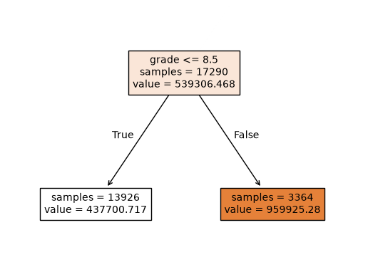

dt.score(X_train, y_train) # Score on the train set

0.3209427041566191

dt.score(X_test, y_test) # Score on the test set

0.31767136668453344

Discuss: are both scores poor, or is only the held-out score poor? What would support calling this underfitting?

Now allow max_depth=20. Predict before running: must both scores improve?

dt = DecisionTreeRegressor(max_depth=20, random_state=RANDOM_STATE)
dt.fit(X_train, y_train)

DecisionTreeRegressor(max_depth=20, random_state=123)

DecisionTreeRegressor

?Documentation for DecisionTreeRegressoriFitted

Parameters

	max_depth max_depth: int, default=None The maximum depth of the tree. If None, then nodes are expanded until all leaves are pure or until all leaves contain less than min_samples_split samples. For an example of how ``max_depth`` influences the model, see :ref:`sphx_glr_auto_examples_tree_plot_tree_regression.py`.	20
	random_state random_state: int, RandomState instance or None, default=None Controls the randomness of the estimator. The features are always randomly permuted at each split, even if ``splitter`` is set to ``"best"``. When ``max_features < n_features``, the algorithm will select ``max_features`` at random at each split before finding the best split among them. But the best found split may vary across different runs, even if ``max_features=n_features``. That is the case, if the improvement of the criterion is identical for several splits and one split has to be selected at random. To obtain a deterministic behaviour during fitting, ``random_state`` has to be fixed to an integer. See :term:`Glossary <random_state>` for details.	123
	criterion criterion: {"squared_error", "absolute_error", "poisson"}, default="squared_error" The function to measure the quality of a split. Supported criteria are "squared_error" for the mean squared error, which is equal to variance reduction as feature selection criterion and minimizes the L2 loss using the mean of each terminal node, "absolute_error" for the mean absolute error, which minimizes the L1 loss using the median of each terminal node, and "poisson" which uses reduction in Poisson deviance to find splits, also using the mean of each terminal node. .. versionadded:: 0.18 Mean Absolute Error (MAE) criterion. .. versionadded:: 0.24 Poisson deviance criterion. .. versionchanged:: 1.9 Criterion `"friedman_mse"` was deprecated.	'squared_error'
	splitter splitter: {"best", "random"}, default="best" The strategy used to choose the split at each node. Supported strategies are "best" to choose the best split and "random" to choose the best random split.	'best'
	min_samples_split min_samples_split: int or float, default=2 The minimum number of samples required to split an internal node: - If int, then consider `min_samples_split` as the minimum number. - If float, then `min_samples_split` is a fraction and `ceil(min_samples_split * n_samples)` are the minimum number of samples for each split. .. versionchanged:: 0.18 Added float values for fractions.	2
	min_samples_leaf min_samples_leaf: int or float, default=1 The minimum number of samples required to be at a leaf node. A split point at any depth will only be considered if it leaves at least ``min_samples_leaf`` training samples in each of the left and right branches. This may have the effect of smoothing the model, especially in regression. - If int, then consider `min_samples_leaf` as the minimum number. - If float, then `min_samples_leaf` is a fraction and `ceil(min_samples_leaf * n_samples)` are the minimum number of samples for each node. .. versionchanged:: 0.18 Added float values for fractions.	1
	min_weight_fraction_leaf min_weight_fraction_leaf: float, default=0.0 The minimum weighted fraction of the sum total of weights (of all the input samples) required to be at a leaf node. Samples have equal weight when sample_weight is not provided.	0.0
	max_features max_features: int, float or {"sqrt", "log2"}, default=None The number of features to consider when looking for the best split: - If int, then consider `max_features` features at each split. - If float, then `max_features` is a fraction and `max(1, int(max_features * n_features_in_))` features are considered at each split. - If "sqrt", then `max_features=sqrt(n_features)`. - If "log2", then `max_features=log2(n_features)`. - If None, then `max_features=n_features`. Note: the search for a split does not stop until at least one valid partition of the node samples is found, even if it requires to effectively inspect more than ``max_features`` features.	None
	max_leaf_nodes max_leaf_nodes: int, default=None Grow a tree with ``max_leaf_nodes`` in best-first fashion. Best nodes are defined as relative reduction in impurity. If None then unlimited number of leaf nodes.	None
	min_impurity_decrease min_impurity_decrease: float, default=0.0 A node will be split if this split induces a decrease of the impurity greater than or equal to this value. The weighted impurity decrease equation is the following:: N_t / N * (impurity - N_t_R / N_t * right_impurity - N_t_L / N_t * left_impurity) where ``N`` is the total number of samples, ``N_t`` is the number of samples at the current node, ``N_t_L`` is the number of samples in the left child, and ``N_t_R`` is the number of samples in the right child. ``N``, ``N_t``, ``N_t_R`` and ``N_t_L`` all refer to the weighted sum, if ``sample_weight`` is passed. .. versionadded:: 0.19	0.0
	ccp_alpha ccp_alpha: non-negative float, default=0.0 Complexity parameter used for Minimal Cost-Complexity Pruning. The subtree with the largest cost complexity that is smaller than ``ccp_alpha`` will be chosen. By default, no pruning is performed. See :ref:`minimal_cost_complexity_pruning` for details. See :ref:`sphx_glr_auto_examples_tree_plot_cost_complexity_pruning.py` for an example of such pruning. .. versionadded:: 0.22	0.0
	monotonic_cst monotonic_cst: array-like of int of shape (n_features), default=None Indicates the monotonicity constraint to enforce on each feature. - 1: monotonic increase - 0: no constraint - -1: monotonic decrease If monotonic_cst is None, no constraints are applied. Monotonicity constraints are not supported for: - multioutput regressions (i.e. when `n_outputs_ > 1`). Read more in the :ref:`User Guide <monotonic_cst_gbdt>`. .. versionadded:: 1.4	None

Fitted attributes

Name	Type	Value
feature_importances_ feature_importances_: ndarray of shape (n_features,) The feature importances. The higher, the more important the feature. The importance of a feature is computed as the (normalized) total reduction of the criterion brought by that feature. It is also known as the Gini importance [4]_. Warning: impurity-based feature importances can be misleading for high cardinality features (many unique values). See :func:`sklearn.inspection.permutation_importance` as an alternative.	ndarray[float64](17,)	[0. ,0.01,0.24,...,0.07,0.03,0.02]
feature_names_in_ feature_names_in_: ndarray of shape (`n_features_in_`,) Names of features seen during :term:`fit`. Defined only when `X` has feature names that are all strings. .. versionadded:: 1.0	ndarray[object](17,)	['bedrooms','bathrooms','sqft_living',...,'long','sqft_living15', 'sqft_lot15']
max_features_ max_features_: int The inferred value of max_features.	int	17
n_features_in_ n_features_in_: int Number of features seen during :term:`fit`. .. versionadded:: 0.24	int	17
n_outputs_ n_outputs_: int The number of outputs when ``fit`` is performed.	int	1
tree_ tree_: Tree instance The underlying Tree object. Please refer to ``help(sklearn.tree._tree.Tree)`` for attributes of Tree object and :ref:`sphx_glr_auto_examples_tree_plot_unveil_tree_structure.py` for basic usage of these attributes.	Tree	<sklearn.tree...t 0x11ce261e0>

dt.score(X_train, y_train) # Score on the train set

0.9968347348881582

dt.score(X_test, y_test) # Score on the test set

0.7378551974307357

Which depth looks more promising? Which dataset just influenced that choice?

Slide pause: underfitting, overfitting, the fundamental trade-off, and the golden rule. Use the exam analogy: learning too little versus memorizing practice-specific details.

Single validation set

We’ve been looking at test scores to compare depths. That turns the test set into part of model selection: it is no longer an independent final assessment.

Let’s introduce a validation set for further choices. This improves our workflow from here onward, but does not make the already-used test set fresh again.

TODO: reserve 20% of X_train, y_train for validation. What fractions of the original data are now used for fitting, validation, and testing?

# TODO: try this step before reading the worked solution below.
# Create a validation set 
X_tr, X_valid, y_tr, y_valid = train_test_split(X_train, y_train, test_size=0.2, random_state=RANDOM_STATE)

# TODO: try this step before reading the worked solution below.
tr_scores = []
valid_scores = []
depths = np.arange(1, 35, 2)

for depth in depths:  
    # Create and fit a decision tree model for the given depth  
    dt = DecisionTreeRegressor(max_depth=depth, random_state=RANDOM_STATE)

    dt.fit(X_tr, y_tr)
    
    # Calculate and append r2 scores on the training and validation sets
    tr_scores.append(dt.score(X_tr, y_tr))    
    valid_scores.append(dt.score(X_valid, y_valid))
    
results_single_valid_df = pd.DataFrame({"train_score": tr_scores, 
                           "valid_score": valid_scores},index = depths)
results_single_valid_df

	train_score	valid_score
1	0.319559	0.326616
3	0.603739	0.555180
5	0.754938	0.677567
7	0.833913	0.737285
9	0.890456	0.763480
11	0.931896	0.790521
13	0.963024	0.769030
15	0.981643	0.752728
17	0.991810	0.735637
19	0.996424	0.745925
21	0.998370	0.734048
23	0.999213	0.741060
25	0.999480	0.722873
27	0.999544	0.723951
29	0.999558	0.734986
31	0.999562	0.724068
33	0.999567	0.724410

# Plot the scores collected above.
results_single_valid_df.plot(
    xlabel="Maximum tree depth",
    ylabel="R² score",
    title="Tree depth and performance on a single validation split",
)
plt.show()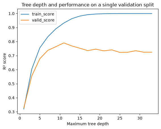

Read the plot together

Where do you see evidence of underfitting or overfitting? Use both scores.
Does extra depth always improve validation performance?
Which depth would you choose?
Would another validation split lead to the same choice?

# TODO: try this step before reading the worked solution below.
# What depth gives the "best" validation score?
best_depth = results_single_valid_df['valid_score'].idxmax() 
best_depth

np.int64(11)

Would another split tell the same story?

Slide pause: five-fold cross-validation. Each configuration is fitted five times, with a different fold held out each time.

TODO: compare the same depths with five-fold CV on X_train, y_train. Record mean training score, mean validation score, and validation-score standard deviation.

Before running: - Does test_score in cross_validate mean our final test set? - How many fits will 17 candidate depths require? - Why use X_train rather than the smaller X_tr?

depths = np.arange(1, 35, 2)
depths

array([ 1,  3,  5,  7,  9, 11, 13, 15, 17, 19, 21, 23, 25, 27, 29, 31, 33])

# TODO: compare depths using five-fold CV (worked solution below).
cv_train_scores = []
cv_valid_scores = []
cv_valid_stds = []

for depth in depths:
    dt = DecisionTreeRegressor(max_depth=depth, random_state=RANDOM_STATE)
    results = cross_validate(
        dt, X_train, y_train, return_train_score=True
    )
    cv_train_scores.append(results['train_score'].mean())
    # Here test_score refers to validation folds, not X_test.
    cv_valid_scores.append(results['test_score'].mean())
    cv_valid_stds.append(results['test_score'].std())

cv_results_df = pd.DataFrame({
    "train_score": cv_train_scores,
    "valid_score": cv_valid_scores,
    "valid_std": cv_valid_stds,
}, index=depths)
cv_results_df.index.name = "max_depth"
cv_results_df

	train_score	valid_score	valid_std
max_depth
1	0.321050	0.322465	0.026939
3	0.603243	0.559284	0.017880
5	0.752169	0.688484	0.015447
7	0.835876	0.758259	0.025574
9	0.894960	0.768184	0.019748
11	0.938201	0.772185	0.022939
13	0.966812	0.760966	0.011522
15	0.983340	0.754620	0.017938
17	0.992220	0.730025	0.036612
19	0.996487	0.722803	0.028504
21	0.998440	0.726659	0.038662
23	0.999178	0.730704	0.015303
25	0.999438	0.711356	0.024054
27	0.999518	0.721917	0.022388
29	0.999539	0.729374	0.013672
31	0.999545	0.740319	0.012144
33	0.999546	0.706489	0.030473

cv_results_df[["train_score", "valid_score"]].plot(
    xlabel="Maximum tree depth",
    ylabel="Mean R² score",
    title="Tree depth and five-fold cross-validation performance",
)
plt.show()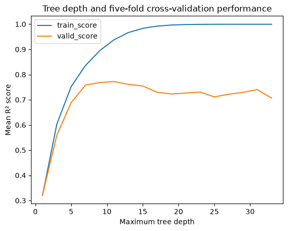

TODO: find the depth with the highest mean CV score. Is a tiny improvement enough to prefer a much deeper tree?

# TODO: try this step before reading the worked solution below.
best_depth = cv_results_df['valid_score'].idxmax()
best_depth

np.int64(11)

❓❓ Questions for you

Discuss the following questions with your neighbour

How does this comparison differ from the single validation split?
How much do validation scores vary across folds? How does that affect your confidence in small differences between depths?
If a shallower tree scores nearly as well as the highest-scoring tree, which would you choose? Explain.
Have we found the best possible depth, or the best choice according to a particular comparison?

Refit the selected configuration and evaluate

Before running: fix your chosen depth and explain why you chose it.

TODO: fit a fresh tree on all non-test training data, then evaluate it on the test set. Why do we refit instead of keeping one of the CV models?

In a fresh workflow, this would be our first look at test performance. Here, we already used these data during EDA and model comparisons, so this score is illustrative—not an independent final estimate. A new independent evaluation would be needed for that claim.

# TODO: record your choice before looking at the final score.
selected_depth = int(best_depth)
selection_reason = "Highest mean validation R² among the depths compared with CV."
print(f"Selected depth: {selected_depth}. {selection_reason}")

# Refit on all non-test training data.
dt_final = DecisionTreeRegressor(max_depth=selected_depth, random_state=RANDOM_STATE)
dt_final.fit(X_train, y_train)
dt_final.score(X_train, y_train)

Selected depth: 11. Highest mean validation R² among the depths compared with CV.

0.9308647034083802

# TODO: try this step before reading the worked solution below.
# Evaluate on the test set
dt_final.score(X_test, y_test)

0.7784948928666875

How does this score compare with the CV estimate? What might explain a difference?

If we now changed the depth because of this score, which role would the test set be playing?

Optional: what features did the tree use?

#What's the depth of the model? 
dt_final.get_depth()

# plot_tree(dt_final, feature_names = X_train.columns.tolist(), impurity=False, filled=True);

# Which features are the most important ones?
dt_final.feature_importances_

array([0.00080741, 0.00327551, 0.25123925, 0.01808825, 0.00079645,
       0.03213916, 0.01190633, 0.00106308, 0.36400802, 0.02313684,
       0.00295235, 0.01209545, 0.00064647, 0.17216105, 0.06835056,
       0.02416048, 0.01317334])

TODO: pair each importance with its feature name and sort the table. Which features does this tree rely on most?

These are impurity-based importances for this fitted tree. They do not establish causation; correlated features can share importance, and features with many possible splits can be favoured. If this exploration motivates another modeling choice, return to validation.

# TODO: try this step before reading the worked solution below.
df = pd.DataFrame( 
    data = {
        "features": dt_final.feature_names_in_,
        "feature_importances": dt_final.feature_importances_
    }
)
df.sort_values("feature_importances", ascending=False)

	features	feature_importances
8	grade	0.364008
2	sqft_living	0.251239
13	lat	0.172161
14	long	0.068351
5	waterfront	0.032139
15	sqft_living15	0.024160
9	sqft_above	0.023137
3	sqft_lot	0.018088
16	sqft_lot15	0.013173
11	yr_built	0.012095
6	view	0.011906
1	bathrooms	0.003276
10	sqft_basement	0.002952
7	condition	0.001063
0	bedrooms	0.000807
4	floors	0.000796
12	yr_renovated	0.000646

Looking back: what did we learn?

Discuss with a neighbour:

Why wasn’t the initial training score enough?
When did our test set start influencing model selection?
Why didn’t creating a validation set later undo that?
What did CV add beyond one validation split?
Where did you see underfitting or overfitting?

The workflow to take away

On a fresh project:

Define the prediction task and reserve a test set using an appropriate split.
Explore the training data and prepare features.
Establish a baseline; compare models and hyperparameters using CV on the training data. Learn any preprocessing within each training fold.
Fix the configuration and refit on all training data.
Evaluate on the untouched test set.
Optionally inspect feature importances to understand the fitted model.

The golden rule: test data must not guide training or model selection.

Our opening shortcuts helped us discover this workflow. They are not steps to copy into a final evaluation.