Chapters 5 and 6: From messy data to a preprocessing pipeline

Can we predict whether someone likes a restaurant from their survey response? In this demo, our task is to predict a respondent’s “like” or “dislike” label from the rest of their restaurant survey response. This is a teaching example for preprocessing mixed data types, rather than a restaurant recommendation system. Comments may directly express the answer, so strong performance does not mean we can predict someone’s preferences before a visit.

We already know how to fit and compare models. Today we will make that workflow work with missing values, different scales, categories, and text.

Recall our machine learning workflow

Define the prediction problem and identify the inputs and target.
Reserve a test set before exploring the data.
Explore the training data and establish a dummy baseline.
Compare models using cross-validation on the training data.
Once choices are settled, refit on all training data and evaluate once on the test set.

Discuss before starting: where does preprocessing belong? What must be learned from training data only?

Our guiding rule: each validation fold must stay unseen while both preprocessing and the model are fitted. We will deliberately show two incorrect cross-validation examples, then repair them with pipelines. The test set stays reserved throughout this demo.

Setup and imports

Run this notebook from content/classes/varada, with this directory’s .venv selected as the kernel. From this directory you can also run:

uv run --locked jupyter lab lecture-05-06-preprocessing-demo.ipynb

The dataset is stored in data/cleaned_restaurant_data.csv. Run cells in order; commented-out failure examples are optional discussion exercises.

from pathlib import Path

import matplotlib.pyplot as plt
import numpy as np
import pandas as pd

from sklearn.compose import ColumnTransformer, make_column_transformer
from sklearn.impute import SimpleImputer
from sklearn.model_selection import cross_val_score, cross_validate, train_test_split
from sklearn.neighbors import KNeighborsClassifier
from sklearn.pipeline import Pipeline, make_pipeline
from sklearn.preprocessing import OneHotEncoder, OrdinalEncoder, StandardScaler

%matplotlib inline

pd.set_option("display.max_colwidth", 200)


DATA_DIR = Path.cwd() / "data"
data_path = DATA_DIR / "cleaned_restaurant_data.csv"
if not data_path.is_file():
    raise FileNotFoundError(
        f"Dataset not found: {data_path}. Start the notebook from content/classes/varada."
    )

Data and splitting

We will use the restaurant survey data. Each row describes one respondent’s restaurant experience. The target is that respondent’s reported like or dislike label, and the inputs are the other fields in their completed survey.

This task asks us to infer a satisfaction label from an existing response. Features such as comments and the assessment of the server describe an experience that has already happened. We are not estimating an intrinsic restaurant rating or learning an individual’s preferences across visits.

Inferring satisfaction could be useful when comments are available but explicit ratings are missing. Here, the survey already collects the label, so the practical value is limited. We use it to learn how to preprocess mixed data types.

Discuss: could a model score well on this task without being useful for deciding where someone should eat next?

df = pd.read_csv(data_path)

# Reserve test rows before inspecting values or choosing cleaning rules.
train_df, test_df = train_test_split(df, test_size=0.2, random_state=123)
train_df.head()

	north_america	eat_out_freq	age	n_people	price	food_type	noise_level	good_server	comments	restaurant_name	target
934	Yes	4.0	21	30.0	30.0	Canadian/American	low	Yes	The building and the room gave a very comfy feeling. Immediately after sitting down it felt like we were right at home.	NaN	like
306	No	8.0	27	NaN	NaN	NaN	NaN	NaN	NaN	NaN	dislike
918	Yes	2.0	23	80.0	40.0	Other	low	Yes	The food was amazing and was extremely unique!	Chambar Restaurant	like
568	Yes	3.0	22	NaN	NaN	NaN	NaN	NaN	NaN	NaN	like
684	No	5.0	22	3.0	12.0	Other	no music	Yes	Tonkatsu number one	Nori	like

❓❓ Questions for you

You have this restaurant dataset. Suppose you want to train a decision tree, KNN, or SVC to predict a respondent’s reported satisfaction label from the other fields in their completed survey.

Can we just call fit on the training data? If not, what hurdles would we face?
Can the model handle NaNs directly?
What to do with strings like food_type?
How to deal with free-form comments?
Do all models care if price and age are on different scales?
Should we keep restaurant_name?
Do we need to encode like/dislike as numbers?

Challenge	Why is it a problem?	Examples from dataset
Missing values	Many ML models in `sklearn` cannot handle NaNs directly	`price`, `food_type`, `noise_level`
Categorical (string) data	Models expect numeric input, not raw strings	`north_america`, `food_type`, `noise_level`
Text features	Free text must be vectorized before use	`comments`
Feature scaling	Features on different scales can distort distance-based models (KNN, SVC)	`age`, `price`, `n_people`, `eat_out_freq`
High-cardinality features	Can overfit or be uninformative if encoded naively	`restaurant_name`
Target encoding	Sklearn allows categorical target labels	`target` (`like` / `dislike`)

Preprocessing is about making the raw dataset ready for machine learning.
We first need to figure out which transformations to apply on which features.

train_df.describe()

	eat_out_freq	age	n_people	price
count	771.000000	771.000000	5.550000e+02	555.000000
mean	2.566550	23.906615	1.804252e+04	1835.646288
std	2.236869	4.408268	4.244753e+05	42446.209043
min	0.000000	10.000000	0.000000e+00	0.000000
25%	1.000000	21.000000	1.000000e+01	17.500000
50%	2.000000	22.000000	2.000000e+01	25.000000
75%	3.000000	26.000000	3.000000e+01	40.000000
max	15.000000	46.000000	1.000000e+07	1000000.000000

Inspect training data and define the demo population

Which values look unusual? A high price is not automatically an error. For this exercise, we restrict the training examples to prices at most 200 and party sizes of at least one, keeping missing values for the imputation lesson. This is a teaching choice, not a general outlier-removal rule.

We leave the test set untouched. A final evaluation would need to state clearly whether it covers all responses or this restricted population.

upperbound_price = 200
lowerbound_people = 1
restaurant_df = train_df.loc[
    ~(train_df['price'] > upperbound_price)
    & ~(train_df['n_people'] < lowerbound_people)
].copy()
restaurant_df.shape

(755, 11)

restaurant_df.describe()

	eat_out_freq	age	n_people	price
count	755.000000	755.000000	539.000000	539.000000
mean	2.581536	23.916556	25.024119	33.346364
std	2.243054	4.427090	22.194087	28.230340
min	0.000000	10.000000	1.000000	0.000000
25%	1.000000	21.000000	10.000000	18.000000
50%	2.000000	22.000000	20.000000	25.000000
75%	3.000000	26.000000	30.000000	40.000000
max	15.000000	46.000000	200.000000	200.000000

Our target is the respondent’s reported like or dislike label for this experience. We exclude target from the inputs and retain the other survey fields for our preprocessing exercises.

X_train = restaurant_df.drop(columns=['target']).copy()
y_train = restaurant_df['target'].copy()
X_test = test_df.drop(columns=['target']).copy()
y_test = test_df['target'].copy()

A controlled teaching modification

We express training prices in cents to make the scale difference more visible. This changes units, not purchasing power. We also assign one training row a rare cuisine label so that a validation fold can contain a category absent from its fitting folds.

These are artificial examples, not data-cleaning recommendations. Any future test or deployment input would need the same price-unit conversion.

X_train['food_type'].value_counts()

food_type
Other                186
Canadian/American    122
Chinese              100
Indian                38
Italian               34
Mexican               20
Fusion                17
Thai                  16
fusion                 6
Name: count, dtype: int64

X_train.loc[X_train.index[0], 'food_type'] = 'Quebecois'
X_train['price'] = X_train['price'] * 100

# Check alignment after filtering training rows.
assert X_train.index.equals(y_train.index)
X_train.shape, X_test.shape

((755, 10), (193, 10))

Exploratory data analysis

X_train.hist(bins=20, figsize=(12, 8));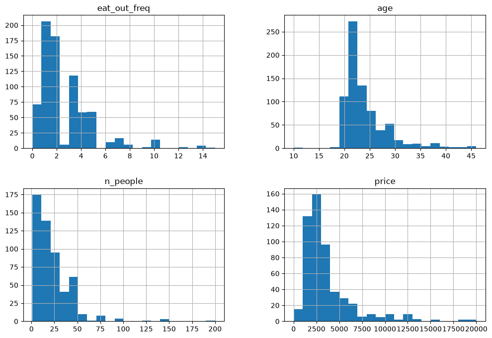

Do you see anything interesting in these plots?

X_train['food_type'].value_counts()

food_type
Other                186
Canadian/American    121
Chinese              100
Indian                38
Italian               34
Mexican               20
Fusion                17
Thai                  16
fusion                 6
Quebecois              1
Name: count, dtype: int64

Error in data collection? Probably “Fusion” and “fusion” categories should be combined?

# Apply a fixed spelling correction identified from training data.
X_train['food_type'] = X_train['food_type'].replace("fusion", "Fusion")

X_train['food_type'].value_counts()

food_type
Other                186
Canadian/American    121
Chinese              100
Indian                38
Italian               34
Fusion                23
Mexican               20
Thai                  16
Quebecois              1
Name: count, dtype: int64

Again, usually we should spend lots of time in EDA, but let’s stop here so that we have time to learn about transformers and pipelines.

Modeling

Establish a dummy baseline

Before using the features, measure how well we can do by always predicting the most frequent training class. We use the same default five-fold classification splits for model comparisons below.

In cross_validate, test_score means the held-out validation fold, not our reserved test set.

from sklearn.dummy import DummyClassifier

dummy = DummyClassifier()
scores = cross_validate(dummy, X_train, y_train, return_train_score=True)
pd.DataFrame(scores)

	fit_time	score_time	test_score	train_score
0	0.000546	0.000349	0.523179	0.518212
1	0.000285	0.000270	0.523179	0.518212
2	0.000268	0.000240	0.516556	0.519868
3	0.000253	0.000232	0.516556	0.519868
4	0.000251	0.000231	0.516556	0.519868

Compare the fold scores with the training target proportions below. What would a useful model need to improve on?

y_train.value_counts(normalize=True)

target
like       0.519205
dislike    0.480795
Name: proportion, dtype: float64

Let’s try KNN on this data

Do you think KNN would work directly on X_train and y_train?

# Preprocessing and pipeline
from sklearn.neighbors import KNeighborsClassifier

knn = KNeighborsClassifier()
# knn.fit(X_train, y_train)

- We need to preprocess the data before feeding it into machine learning models. What are the different types of features in the data? - What transformations are necessary before training a machine learning model? - Can we categorize features based on the type of transformations they require?

X_train[4:11]

	north_america	eat_out_freq	age	n_people	price	food_type	noise_level	good_server	comments	restaurant_name
684	No	5.0	22	3.0	1200.0	Other	no music	Yes	Tonkatsu number one	Nori
97	Yes	2.0	26	25.0	3500.0	Italian	high	No	seated at a very crowded area, didn't take our orders until 20 min later	NaN
864	No	3.0	25	NaN	NaN	NaN	NaN	NaN	NaN	NaN
779	Yes	5.0	20	NaN	NaN	NaN	NaN	NaN	NaN	NaN
848	Yes	1.0	21	NaN	NaN	NaN	NaN	NaN	NaN	NaN
392	Yes	2.0	22	30.0	2500.0	Other	high	Yes	temperature in the restaurant	Don't remember
883	Yes	2.0	26	45.0	3500.0	Chinese	medium	Yes	Fresh food, great taste, great service, great value for money	Hotpot on Broadway

numeric_feats = ['age', 'n_people', 'price'] # Continuous and quantitative features
categorical_feats = ['food_type', 'north_america'] # Discrete and qualitative features
binary_feats = ['good_server'] # Categorical features with only two possible values 
ordinal_feats = ['noise_level'] # Some natural ordering in the categories 
noise_cats = ['no music', 'low', 'medium', 'high', 'crazy loud']
drop_feats = ['comments', 'restaurant_name', 'eat_out_freq'] # Omit these for now to focus on preprocessing; revisit comments later

X_train['north_america'].value_counts()

north_america
Yes                    404
No                     343
Don't want to share      8
Name: count, dtype: int64

X_train['good_server'].value_counts()

good_server
Yes    392
No     142
Name: count, dtype: int64

X_train.columns

Index(['north_america', 'eat_out_freq', 'age', 'n_people', 'price',
       'food_type', 'noise_level', 'good_server', 'comments',
       'restaurant_name'],
      dtype='str')

X_train['food_type'].value_counts()

food_type
Other                186
Canadian/American    121
Chinese              100
Indian                38
Italian               34
Fusion                23
Mexican               20
Thai                  16
Quebecois              1
Name: count, dtype: int64

X_train['north_america'].value_counts()

north_america
Yes                    404
No                     343
Don't want to share      8
Name: count, dtype: int64

X_train['good_server'].value_counts()

good_server
Yes    392
No     142
Name: count, dtype: int64

X_train['noise_level'].value_counts()

noise_level
medium        230
low           174
high           74
no music       41
crazy loud     20
Name: count, dtype: int64

Start with numerical features

Let’s build a KNN classifier using just age, n_people, and price. We will work through four steps:

Find the missing values.
Fill them using an imputer.
Scale the features so their units do not dominate distances.
Evaluate all these steps together using a pipeline.

For now, we use only training data. First we will inspect how the transformations work; then we will work out how to evaluate them correctly.

1. Can KNN use these columns as they are?

These columns are numerical, but that does not mean they are ready for KNN. Inspect a few rows, then count the missing values in each column.

X_train_num = X_train[numeric_feats].copy()
X_train_num.head()

	age	n_people	price
934	21	30.0	3000.0
306	27	NaN	NaN
918	23	80.0	4000.0
568	22	NaN	NaN
684	22	3.0	1200.0

X_train_num.isna().sum()

age           0
n_people    216
price       216
dtype: int64

Discuss: how would KNN calculate a distance if one of the coordinates were missing?

KNN cannot fit data containing NaN. The commented line below is an optional failure example. We need to fill the missing values before fitting.

knn = KNeighborsClassifier()
# Optional: uncomment to see the missing-value error.
# knn.fit(X_train_num, y_train)

2. Fill missing values with `SimpleImputer`

We will replace missing values with the median of their column. This involves two different operations:

fit: learn one median per column from the fitting rows.
transform: fill missing entries using those stored medians, leaving observed entries unchanged.

First, inspect the values the imputer learns. These medians come from all training rows for this demonstration of the mechanics; we have not started cross-validation yet.

imputer = SimpleImputer(strategy="median")
imputer.fit(X_train_num)

pd.Series(imputer.statistics_, index=numeric_feats, name="Learned median")

age           22.0
n_people      20.0
price       2500.0
Name: Learned median, dtype: float64

X_train_num_imp = imputer.transform(X_train_num)

# Restore column names and row labels to inspect the returned array.
imputed_df = pd.DataFrame(
    X_train_num_imp, columns=numeric_feats, index=X_train_num.index
)
imputed_df.head()

	age	n_people	price
934	21.0	30.0	3000.0
306	27.0	20.0	2500.0
918	23.0	80.0	4000.0
568	22.0	20.0	2500.0
684	22.0	3.0	1200.0

# Every numerical column should now have zero missing values.
imputed_df.isna().sum()

age         0
n_people    0
price       0
dtype: int64

Check your understanding: if a new row has a missing price, do we calculate a new median or use the stored price median?

Use the stored median. New rows are transformed using what was learned during fitting.

KNN can now fit. The score below is training accuracy, so it only describes predictions on examples the model has already seen.

knn.fit(X_train_num_imp, y_train)
knn.score(X_train_num_imp, y_train)

0.6701986754966888

We have solved the missing-value problem. We have not yet measured generalization, and this training score is not a fair comparison with the dummy model’s validation score. Before evaluating, there is one more issue with our distances.

3. Put the numerical features on comparable scales

Earlier, we expressed price in cents. A price difference of 1,000 cents contributes much more to squared Euclidean distance than an age difference of 10 years. Changing currency units should not decide which neighbours matter most.

Inspect the ranges below. Which feature could dominate distance before scaling?

imputed_df.describe().loc[["mean", "std", "min", "max"]]

	age	n_people	price
mean	23.916556	23.586755	3095.852980
std	4.427090	18.884652	2414.320499
min	10.000000	1.000000	0.000000
max	46.000000	200.000000	20000.000000

StandardScaler subtracts each column’s learned mean and divides by its learned standard deviation:

\[z = \frac{x - \mu}{\sigma}\]

It follows the same pattern as the imputer: fit to learn, transform to apply. We scale after imputation so we work with a complete numerical matrix.

scaler = StandardScaler()
scaler.fit(X_train_num_imp)
X_train_num_imp_scaled = scaler.transform(X_train_num_imp)

scaled_df = pd.DataFrame(
    X_train_num_imp_scaled, columns=numeric_feats, index=X_train_num.index
)
scaled_df.head()

	age	n_people	price
934	-0.659234	0.339826	-0.039728
306	0.696956	-0.190056	-0.246963
918	-0.207171	2.989234	0.374742
568	-0.433203	-0.190056	-0.246963
684	-0.433203	-1.090854	-0.785774

# On these fitting rows, means should be about 0 and standard deviations about 1.
pd.DataFrame({
    "mean": scaled_df.mean(),
    "std": scaled_df.std(ddof=0),
}).round(3)

	mean	std
age	-0.0	1.0
n_people	0.0	1.0
price	0.0	1.0

Negative values now mean “below the fitting-data mean”, not negative ages or prices. Scaling changes the representation, not the original measurements.

Discuss: would converting dollars to cents still change these standardized values? Would scaling necessarily improve validation accuracy?

Both the imputer and scaler are transformers: they learn with fit and apply a transformation with transform. KNN is a predictor: it learns with fit and predicts labels with predict. All three are estimators.

4. Evaluate the whole procedure

Our proposed procedure is now impute \(\to\) scale \(\to\) fit KNN. How should we cross-validate it?

The next cell is deliberately incorrect, even though it runs. Before running it, ask: which rows have already influenced the medians, means, and standard deviations?

# Incorrect evaluation: preprocessing was fitted before the CV folds were created.
leaky_cv_scores = cross_val_score(knn, X_train_num_imp_scaled, y_train, cv=5)
leaky_cv_scores

array([0.50993377, 0.52317881, 0.49006623, 0.53642384, 0.54304636])

Cross-validation splits the matrix it receives. Here, the imputer and scaler have already learned from every training row, including the rows that will become validation folds.

That leaks information across folds. The final test set is still separate, but each validation fold was supposed to be unseen too. The procedure is incorrect even if the effect on the scores is small.

Repair it: split into folds first; within each fold, fit the imputer, scaler, and KNN using only the fitting rows. Apply those learned transformations to the validation rows.

Let a pipeline keep the steps together

A pipeline packages the transformations and model into a single estimator. Pass the pipeline and the raw numerical columns to cross-validation. Each fold then fits a fresh copy of all three steps.

pipe_knn = make_pipeline(
    SimpleImputer(strategy="median"),
    StandardScaler(),
    KNeighborsClassifier(),
)
pipe_knn

Pipeline(steps=[('simpleimputer', SimpleImputer(strategy='median')),
                ('standardscaler', StandardScaler()),
                ('kneighborsclassifier', KNeighborsClassifier())])

In a Jupyter environment, please rerun this cell to show the HTML representation or trust the notebook.
On GitHub, the HTML representation is unable to render, please try loading this page with nbviewer.org.

pipe_knn.fit(X_train_num, y_train)

Pipeline(steps=[('simpleimputer', SimpleImputer(strategy='median')),
                ('standardscaler', StandardScaler()),
                ('kneighborsclassifier', KNeighborsClassifier())])

Pipeline

?Documentation for PipelineiFitted

Parameters

	steps steps: list of tuples List of (name of step, estimator) tuples that are to be chained in sequential order. To be compatible with the scikit-learn API, all steps must define `fit`. All non-last steps must also define `transform`. See :ref:`Combining Estimators <combining_estimators>` for more details.	[('simpleimputer', ...), ('standardscaler', ...), ...]
	transform_input transform_input: list of str, default=None The names of the :term:`metadata` parameters that should be transformed by the pipeline before passing it to the step consuming it. This enables transforming some input arguments to ``fit`` (other than ``X``) to be transformed by the steps of the pipeline up to the step which requires them. Requirement is defined via :ref:`metadata routing <metadata_routing>`. For instance, this can be used to pass a validation set through the pipeline. You can only set this if metadata routing is enabled, which you can enable using ``sklearn.set_config(enable_metadata_routing=True)``. .. versionadded:: 1.6	None
	memory memory: str or object with the joblib.Memory interface, default=None Used to cache the fitted transformers of the pipeline. The last step will never be cached, even if it is a transformer. By default, no caching is performed. If a string is given, it is the path to the caching directory. Enabling caching triggers a clone of the transformers before fitting. Therefore, the transformer instance given to the pipeline cannot be inspected directly. Use the attribute ``named_steps`` or ``steps`` to inspect estimators within the pipeline. Caching the transformers is advantageous when fitting is time consuming. See :ref:`sphx_glr_auto_examples_neighbors_plot_caching_nearest_neighbors.py` for an example on how to enable caching.	None
	verbose verbose: bool, default=False If True, the time elapsed while fitting each step will be printed as it is completed.	False

Fitted attributes

Name	Type	Value
classes_ classes_: ndarray of shape (n_classes,) The classes labels. Only exist if the last step of the pipeline is a classifier.	ndarray[object](2,)	['dislike','like']
feature_names_in_ feature_names_in_: ndarray of shape (`n_features_in_`,) Names of features seen during :term:`fit`. Only defined if the underlying estimator exposes such an attribute when fit. .. versionadded:: 1.0	ndarray[object](3,)	['age','n_people','price']
n_features_in_ n_features_in_: int Number of features seen during :term:`fit`. Only defined if the underlying first estimator in `steps` exposes such an attribute when fit. .. versionadded:: 0.24	int	3

SimpleImputer

?Documentation for SimpleImputer

Parameters

	strategy strategy: str or Callable, default='mean' The imputation strategy. - If "mean", then replace missing values using the mean along each column. Can only be used with numeric data. - If "median", then replace missing values using the median along each column. Can only be used with numeric data. - If "most_frequent", then replace missing using the most frequent value along each column. Can be used with strings or numeric data. If there is more than one such value, only the smallest is returned. - If "constant", then replace missing values with fill_value. Can be used with strings or numeric data. - If an instance of Callable, then replace missing values using the scalar statistic returned by running the callable over a dense 1d array containing non-missing values of each column. .. versionadded:: 0.20 strategy="constant" for fixed value imputation. .. versionadded:: 1.5 strategy=callable for custom value imputation.	'median'
	missing_values missing_values: int, float, str, np.nan, None or pandas.NA, default=np.nan The placeholder for the missing values. All occurrences of `missing_values` will be imputed. For pandas' dataframes with nullable integer dtypes with missing values, `missing_values` can be set to either `np.nan` or `pd.NA`.	nan
	fill_value fill_value: str or numerical value, default=None When strategy == "constant", `fill_value` is used to replace all occurrences of missing_values. For string or object data types, `fill_value` must be a string. If `None`, `fill_value` will be 0 when imputing numerical data and "missing_value" for strings or object data types.	None
	copy copy: bool, default=True If True, a copy of X will be created. If False, imputation will be done in-place whenever possible. Note that, in the following cases, a new copy will always be made, even if `copy=False`: - If `X` is not an array of floating values; - If `X` is encoded as a CSR matrix; - If `add_indicator=True`.	True
	add_indicator add_indicator: bool, default=False If True, a :class:`MissingIndicator` transform will stack onto output of the imputer's transform. This allows a predictive estimator to account for missingness despite imputation. If a feature has no missing values at fit/train time, the feature won't appear on the missing indicator even if there are missing values at transform/test time.	False
	keep_empty_features keep_empty_features: bool, default=False If True, features that consist exclusively of missing values when `fit` is called are returned in results when `transform` is called. The imputed value is always `0` except when `strategy="constant"` in which case `fill_value` will be used instead. .. versionadded:: 1.2	False

Fitted attributes

Name	Type	Value
feature_names_in_ feature_names_in_: ndarray of shape (`n_features_in_`,) Names of features seen during :term:`fit`. Defined only when `X` has feature names that are all strings. .. versionadded:: 1.0	ndarray[object](3,)	['age','n_people','price']
indicator_ indicator_: :class:`~sklearn.impute.MissingIndicator` Indicator used to add binary indicators for missing values. `None` if `add_indicator=False`.	NoneType	None
n_features_in_ n_features_in_: int Number of features seen during :term:`fit`. .. versionadded:: 0.24	int	3
statistics_ statistics_: array of shape (n_features,) The imputation fill value for each feature. Computing statistics can result in `np.nan` values. During :meth:`transform`, features corresponding to `np.nan` statistics will be discarded.	ndarray[float64](3,)	[ 22., 20.,2500.]

3 features

age
n_people
price

StandardScaler

?Documentation for StandardScaler

Parameters

	copy copy: bool, default=True If False, try to avoid a copy and do inplace scaling instead. This is not guaranteed to always work inplace; e.g. if the data is not a NumPy array or scipy.sparse CSR matrix, a copy may still be returned.	True
	with_mean with_mean: bool, default=True If True, center the data before scaling. This does not work (and will raise an exception) when attempted on sparse matrices, because centering them entails building a dense matrix which in common use cases is likely to be too large to fit in memory.	True
	with_std with_std: bool, default=True If True, scale the data to unit variance (or equivalently, unit standard deviation).	True

Fitted attributes

Name	Type	Value
mean_ mean_: ndarray of shape (n_features,) or None The mean value for each feature in the training set. Equal to ``None`` when ``with_mean=False`` and ``with_std=False``.	ndarray[float64](3,)	[ 23.92, 23.59,3095.85]
n_features_in_ n_features_in_: int Number of features seen during :term:`fit`. .. versionadded:: 0.24	int	3
n_samples_seen_ n_samples_seen_: int or ndarray of shape (n_features,) The number of samples processed by the estimator for each feature. If there are no missing samples, the ``n_samples_seen`` will be an integer, otherwise it will be an array of dtype int. If `sample_weights` are used it will be a float (if no missing data) or an array of dtype float that sums the weights seen so far. Will be reset on new calls to fit, but increments across ``partial_fit`` calls.	float64	755
scale_ scale_: ndarray of shape (n_features,) or None Per feature relative scaling of the data to achieve zero mean and unit variance. Generally this is calculated using `np.sqrt(var_)`. If a variance is zero, we can't achieve unit variance, and the data is left as-is, giving a scaling factor of 1. `scale_` is equal to `None` when `with_std=False`. .. versionadded:: 0.17 scale_	ndarray[float64](3,)	[ 4.42, 18.87,2412.72]
var_ var_: ndarray of shape (n_features,) or None The variance for each feature in the training set. Used to compute `scale_`. Equal to ``None`` when ``with_mean=False`` and ``with_std=False``.	ndarray[float64](3,)	[ 19.57, 356.16,5821223.02]

3 features

x0
x1
x2

KNeighborsClassifier

?Documentation for KNeighborsClassifier

Parameters

	n_neighbors n_neighbors: int, default=5 Number of neighbors to use by default for :meth:`kneighbors` queries.	5
	weights weights: {'uniform', 'distance'}, callable or None, default='uniform' Weight function used in prediction. Possible values: - 'uniform' : uniform weights. All points in each neighborhood are weighted equally. - 'distance' : weight points by the inverse of their distance. in this case, closer neighbors of a query point will have a greater influence than neighbors which are further away. - [callable] : a user-defined function which accepts an array of distances, and returns an array of the same shape containing the weights. Refer to the example entitled :ref:`sphx_glr_auto_examples_neighbors_plot_classification.py` showing the impact of the `weights` parameter on the decision boundary.	'uniform'
	algorithm algorithm: {'auto', 'ball_tree', 'kd_tree', 'brute'}, default='auto' Algorithm used to compute the nearest neighbors: - 'ball_tree' will use :class:`BallTree` - 'kd_tree' will use :class:`KDTree` - 'brute' will use a brute-force search. - 'auto' will attempt to decide the most appropriate algorithm based on the values passed to :meth:`fit` method. Note: fitting on sparse input will override the setting of this parameter, using brute force.	'auto'
	leaf_size leaf_size: int, default=30 Leaf size passed to BallTree or KDTree. This can affect the speed of the construction and query, as well as the memory required to store the tree. The optimal value depends on the nature of the problem.	30
	p p: float, default=2 Power parameter for the Minkowski metric. When p = 1, this is equivalent to using manhattan_distance (l1), and euclidean_distance (l2) for p = 2. For arbitrary p, minkowski_distance (l_p) is used. This parameter is expected to be positive.	2
	metric metric: str or callable, default='minkowski' Metric to use for distance computation. Default is "minkowski", which results in the standard Euclidean distance when p = 2. See the documentation of `scipy.spatial.distance <https://docs.scipy.org/doc/scipy/reference/spatial.distance.html>`_ and the metrics listed in :class:`~sklearn.metrics.pairwise.distance_metrics` for valid metric values. If metric is "precomputed", X is assumed to be a distance matrix and must be square during fit. X may be a :term:`sparse graph`, in which case only "nonzero" elements may be considered neighbors. If metric is a callable function, it takes two arrays representing 1D vectors as inputs and must return one value indicating the distance between those vectors. This works for Scipy's metrics, but is less efficient than passing the metric name as a string.	'minkowski'
	metric_params metric_params: dict, default=None Additional keyword arguments for the metric function.	None
	n_jobs n_jobs: int, default=None The number of parallel jobs to run for neighbors search. ``None`` means 1 unless in a :obj:`joblib.parallel_backend` context. ``-1`` means using all processors. See :term:`Glossary <n_jobs>` for more details. Doesn't affect :meth:`fit` method.	None

Fitted attributes

Name	Type	Value
classes_ classes_: array of shape (n_classes,) Class labels known to the classifier	ndarray[object](2,)	['dislike','like']
effective_metric_ effective_metric_: str or callble The distance metric used. It will be same as the `metric` parameter or a synonym of it, e.g. 'euclidean' if the `metric` parameter set to 'minkowski' and `p` parameter set to 2.	str	'eu...an'
effective_metric_params_ effective_metric_params_: dict Additional keyword arguments for the metric function. For most metrics will be same with `metric_params` parameter, but may also contain the `p` parameter value if the `effective_metric_` attribute is set to 'minkowski'.	dict	{}
n_features_in_ n_features_in_: int Number of features seen during :term:`fit`. .. versionadded:: 0.24	int	3
n_samples_fit_ n_samples_fit_: int Number of samples in the fitted data.	int	755
outputs_2d_ outputs_2d_: bool False when `y`'s shape is (n_samples, ) or (n_samples, 1) during fit otherwise True.	bool	False

cross_val_score(pipe_knn, X_train_num, y_train)

array([0.49668874, 0.54304636, 0.49006623, 0.54304636, 0.53642384])

Within each CV fold:

Step	Fitting rows	Validation rows
Imputer	Learn medians and fill missing entries	Fill using the stored medians
Scaler	Learn means/scales and standardize	Standardize using the stored means/scales
KNN	Fit on transformed rows	Predict and calculate accuracy

The next comparison uses the same five-fold splits for the dummy baseline and numerical-feature KNN pipeline. Here, test_score means validation-fold accuracy, not a score on our reserved test set.

numeric_cv_results = cross_validate(
    pipe_knn, X_train_num, y_train, cv=5, return_train_score=True
)
dummy_numeric_cv_results = cross_validate(
    DummyClassifier(), X_train_num, y_train, cv=5, return_train_score=True
)

pd.DataFrame({
    name: {
        "Mean training accuracy": result["train_score"].mean(),
        "Mean validation accuracy": result["test_score"].mean(),
        "Validation accuracy std": result["test_score"].std(),
    }
    for name, result in {
        "Dummy baseline": dummy_numeric_cv_results,
        "Numerical KNN pipeline": numeric_cv_results,
    }.items()
}).T

	Mean training accuracy	Mean validation accuracy	Validation accuracy std
Dummy baseline	0.519205	0.519205	0.003244
Numerical KNN pipeline	0.660265	0.521854	0.023470

Pause and connect the steps

Does the numerical-feature pipeline improve on the dummy baseline on validation folds?
Why did we pass X_train_num, rather than X_train_num_imp_scaled, to cross-validation?
What gets learned again in each fold?

Takeaway: preprocessing is part of the model-fitting procedure. Cross-validate the whole pipeline, not just the final classifier.

We can now handle missing numerical values and different scales. Next, we will apply the same pattern to categorical features: choose a representation, inspect it, and put the transformation inside a pipeline.

Categorical features: represent names without inventing an order

Would coding cuisines as 0, 1, 2 give KNN a meaningful distance? One-hot encoding gives each category its own indicator column.

We first inspect the representation, then put the encoder inside a pipeline. Watch for a category that appears only in a validation fold.

X_train['food_type'].value_counts()

food_type
Other                186
Canadian/American    121
Chinese              100
Indian                38
Italian               34
Fusion                23
Mexican               20
Thai                  16
Quebecois              1
Name: count, dtype: int64

X_train[categorical_feats]

	food_type	north_america
934	Quebecois	Yes
306	NaN	No
918	Other	Yes
568	NaN	Yes
684	Other	No
...	...	...
98	Mexican	No
322	NaN	Yes
382	Italian	No
365	NaN	No
510	Canadian/American	No

755 rows × 2 columns

X_train['north_america'].value_counts()

north_america
Yes                    404
No                     343
Don't want to share      8
Name: count, dtype: int64

X_train['food_type'].value_counts()

food_type
Other                186
Canadian/American    121
Chinese              100
Indian                38
Italian               34
Fusion                23
Mexican               20
Thai                  16
Quebecois              1
Name: count, dtype: int64

X_train_cat = X_train[categorical_feats]

ohe = OneHotEncoder(sparse_output=False)
X_train_cat_ohe = ohe.fit_transform(X_train_cat)

X_train_cat_ohe

array([[0., 0., 0., ..., 0., 0., 1.],
       [0., 0., 0., ..., 0., 1., 0.],
       [0., 0., 0., ..., 0., 0., 1.],
       ...,
       [0., 0., 0., ..., 0., 1., 0.],
       [0., 0., 0., ..., 0., 1., 0.],
       [1., 0., 0., ..., 0., 1., 0.]], shape=(755, 13))

This is a dense array because we set sparse_output=False. Most indicator entries are zero: why might sparse output save memory when there are many categories?

# Get the OHE feature names 

ohe_feats = ohe.get_feature_names_out().tolist()
ohe_feats

['food_type_Canadian/American',
 'food_type_Chinese',
 'food_type_Fusion',
 'food_type_Indian',
 'food_type_Italian',
 'food_type_Mexican',
 'food_type_Other',
 'food_type_Quebecois',
 'food_type_Thai',
 'food_type_nan',
 "north_america_Don't want to share",
 'north_america_No',
 'north_america_Yes']

pd.DataFrame(X_train_cat_ohe, columns = ohe_feats)

	food_type_Canadian/American	food_type_Chinese	food_type_Fusion	food_type_Indian	food_type_Italian	food_type_Mexican	food_type_Other	food_type_Quebecois	food_type_Thai	food_type_nan	north_america_Don't want to share	north_america_No	north_america_Yes
0	0.0	0.0	0.0	0.0	0.0	0.0	0.0	1.0	0.0	0.0	0.0	0.0	1.0
1	0.0	0.0	0.0	0.0	0.0	0.0	0.0	0.0	0.0	1.0	0.0	1.0	0.0
2	0.0	0.0	0.0	0.0	0.0	0.0	1.0	0.0	0.0	0.0	0.0	0.0	1.0
3	0.0	0.0	0.0	0.0	0.0	0.0	0.0	0.0	0.0	1.0	0.0	0.0	1.0
4	0.0	0.0	0.0	0.0	0.0	0.0	1.0	0.0	0.0	0.0	0.0	1.0	0.0
...	...	...	...	...	...	...	...	...	...	...	...	...	...
750	0.0	0.0	0.0	0.0	0.0	1.0	0.0	0.0	0.0	0.0	0.0	1.0	0.0
751	0.0	0.0	0.0	0.0	0.0	0.0	0.0	0.0	0.0	1.0	0.0	0.0	1.0
752	0.0	0.0	0.0	0.0	1.0	0.0	0.0	0.0	0.0	0.0	0.0	1.0	0.0
753	0.0	0.0	0.0	0.0	0.0	0.0	0.0	0.0	0.0	1.0	0.0	1.0	0.0
754	1.0	0.0	0.0	0.0	0.0	0.0	0.0	0.0	0.0	0.0	0.0	1.0	0.0

755 rows × 13 columns

# Deliberately incorrect: the encoder saw all rows before CV split them.
cross_val_score(knn, X_train_cat_ohe, y_train)

array([0.54966887, 0.52980132, 0.49668874, 0.53642384, 0.49006623])

Find the leak again: which rows determined the encoder’s vocabulary?

Now move encoding inside CV. What happens if a validation cuisine was absent from the fitting rows? handle_unknown="ignore" represents it with zeros in that feature’s indicator columns.

Use an imputer and encoder inside the pipeline so missing-value handling and category learning both happen within each fitting fold.

# Code to create a pipeline for OHE and KNN
pipe_ohe_knn = make_pipeline(
    SimpleImputer(strategy="most_frequent"),
    OneHotEncoder(sparse_output=False, handle_unknown="ignore"),
    KNeighborsClassifier()
)

cross_val_score(pipe_ohe_knn, X_train_cat, y_train)

array([0.54966887, 0.52980132, 0.49006623, 0.58940397, 0.50993377])

Ordinal features: use a meaningful order

Noise levels have a natural order. We specify that order explicitly rather than letting alphabetical order decide it. Encoding levels as consecutive integers also imposes equal spacing for KNN: is that a reasonable simplification?

noise_ordering = ['no music', 'low', 'medium', 'high', 'crazy loud']

X_train['noise_level'].value_counts()

noise_level
medium        230
low           174
high           74
no music       41
crazy loud     20
Name: count, dtype: int64

pipe_ordinal_knn = make_pipeline(
    OrdinalEncoder(categories=[noise_ordering]),
    KNeighborsClassifier()
)

# Optional intentional failure: missing noise levels still need imputation.
# cross_val_score(pipe_ordinal_knn, X_train[["noise_level"]], y_train)

X_train['noise_level'].isnull().any()

np.True_

There are missing values. So we need an imputer.

from sklearn.preprocessing import OrdinalEncoder
noise_ordering = ['no music', 'low', 'medium', 'high', 'crazy loud']

ordinal_transformer = make_pipeline(
    SimpleImputer(strategy="most_frequent"),
    OrdinalEncoder(categories=[noise_ordering]),
    KNeighborsClassifier()
)

cross_val_score(ordinal_transformer, X_train[['noise_level']], y_train)

array([0.61589404, 0.56953642, 0.55629139, 0.55629139, 0.55629139])

Combine the feature groups with `ColumnTransformer`

We have explored each feature type separately. Now apply the appropriate transformation to each group and join the resulting columns into one feature matrix. A ColumnTransformer handles the columns; an outer pipeline connects preprocessing to the classifier.

How can we horizontally stack
- preprocessed numeric features, - preprocessed binary features, - preprocessed ordinal features, and - preprocessed categorical features?

Let’s define a column transformer.

from sklearn.compose import make_column_transformer

numeric_transformer = make_pipeline(SimpleImputer(strategy="median"),
                                    StandardScaler()) 
binary_transformer = make_pipeline(SimpleImputer(strategy="most_frequent"), 
                                    OneHotEncoder(drop="if_binary"))
ordinal_transformer = make_pipeline(SimpleImputer(strategy="most_frequent"), 
                                    OrdinalEncoder(categories=[noise_ordering]))
categorical_transformer = make_pipeline(SimpleImputer(strategy="most_frequent"), 
                                    OneHotEncoder(sparse_output=False, handle_unknown="ignore"))

# Define the column transformer
preprocessor = make_column_transformer(
    (numeric_transformer, numeric_feats),
    (binary_transformer, binary_feats),
    (ordinal_transformer, ordinal_feats),
    (categorical_transformer, categorical_feats),    
    ("drop", drop_feats), 
    verbose_feature_names_out = False
)

How does the transformed data look like?

categorical_feats

['food_type', 'north_america']

X_train.shape

(755, 10)

transformed = preprocessor.fit_transform(X_train)
transformed.shape

(755, 17)

preprocessor

ColumnTransformer(transformers=[('pipeline-1',
                                 Pipeline(steps=[('simpleimputer',
                                                  SimpleImputer(strategy='median')),
                                                 ('standardscaler',
                                                  StandardScaler())]),
                                 ['age', 'n_people', 'price']),
                                ('pipeline-2',
                                 Pipeline(steps=[('simpleimputer',
                                                  SimpleImputer(strategy='most_frequent')),
                                                 ('onehotencoder',
                                                  OneHotEncoder(drop='if_binary'))]),
                                 ['good_server']),
                                ('pipeline-3',...
                                                                              'low',
                                                                              'medium',
                                                                              'high',
                                                                              'crazy '
                                                                              'loud']]))]),
                                 ['noise_level']),
                                ('pipeline-4',
                                 Pipeline(steps=[('simpleimputer',
                                                  SimpleImputer(strategy='most_frequent')),
                                                 ('onehotencoder',
                                                  OneHotEncoder(handle_unknown='ignore',
                                                                sparse_output=False))]),
                                 ['food_type', 'north_america']),
                                ('drop', 'drop',
                                 ['comments', 'restaurant_name',
                                  'eat_out_freq'])],
                  verbose_feature_names_out=False)

ColumnTransformer

?Documentation for ColumnTransformeriFitted

Parameters

	transformers transformers: list of tuples List of (name, transformer, columns) tuples specifying the transformer objects to be applied to subsets of the data. name : str Like in Pipeline and FeatureUnion, this allows the transformer and its parameters to be set using ``set_params`` and searched in grid search. transformer : {'drop', 'passthrough'} or estimator Estimator must support :term:`fit` and :term:`transform`. Special-cased strings 'drop' and 'passthrough' are accepted as well, to indicate to drop the columns or to pass them through untransformed, respectively. columns : str, array-like of str, int, array-like of int, array-like of bool, slice or callable Indexes the data on its second axis. Integers are interpreted as positional columns, while strings can reference DataFrame columns by name. A scalar string or int should be used where ``transformer`` expects X to be a 1d array-like (vector), otherwise a 2d array will be passed to the transformer. A callable is passed the input data `X` and can return any of the above. To select multiple columns by name or dtype, you can use :obj:`make_column_selector`.	[('pipeline-1', ...), ('pipeline-2', ...), ...]
	verbose_feature_names_out verbose_feature_names_out: bool, str or Callable[[str, str], str], default=True - If True, :meth:`ColumnTransformer.get_feature_names_out` will prefix all feature names with the name of the transformer that generated that feature. It is equivalent to setting `verbose_feature_names_out="{transformer_name}__{feature_name}"`. - If False, :meth:`ColumnTransformer.get_feature_names_out` will not prefix any feature names and will error if feature names are not unique. - If ``Callable[[str, str], str]``, :meth:`ColumnTransformer.get_feature_names_out` will rename all the features using the name of the transformer. The first argument of the callable is the transformer name and the second argument is the feature name. The returned string will be the new feature name. - If ``str``, it must be a string ready for formatting. The given string will be formatted using two field names: ``transformer_name`` and ``feature_name``. e.g. ``"{feature_name}__{transformer_name}"``. See :meth:`str.format` method from the standard library for more info. .. versionadded:: 1.0 .. versionchanged:: 1.6 `verbose_feature_names_out` can be a callable or a string to be formatted.	False
	remainder remainder: {'drop', 'passthrough'} or estimator, default='drop' By default, only the specified columns in `transformers` are transformed and combined in the output, and the non-specified columns are dropped. (default of ``'drop'``). By specifying ``remainder='passthrough'``, all remaining columns that were not specified in `transformers`, but present in the data passed to `fit` will be automatically passed through. This subset of columns is concatenated with the output of the transformers. For dataframes, extra columns not seen during `fit` will be excluded from the output of `transform`. By setting ``remainder`` to be an estimator, the remaining non-specified columns will use the ``remainder`` estimator. The estimator must support :term:`fit` and :term:`transform`. Note that using this feature requires that the DataFrame columns input at :term:`fit` and :term:`transform` have identical order.	'drop'
	sparse_threshold sparse_threshold: float, default=0.3 If the output of the different transformers contains sparse matrices, these will be stacked as a sparse matrix if the overall density is lower than this value. Use ``sparse_threshold=0`` to always return dense. When the transformed output consists of all dense data, the stacked result will be dense, and this keyword will be ignored.	0.3
	n_jobs n_jobs: int, default=None Number of jobs to run in parallel. ``None`` means 1 unless in a :obj:`joblib.parallel_backend` context. ``-1`` means using all processors. See :term:`Glossary <n_jobs>` for more details.	None
	transformer_weights transformer_weights: dict, default=None Multiplicative weights for features per transformer. The output of the transformer is multiplied by these weights. Keys are transformer names, values the weights.	None
	verbose verbose: bool, default=False If True, the time elapsed while fitting each transformer will be printed as it is completed.	False

Fitted attributes

Name	Type	Value
feature_names_in_ feature_names_in_: ndarray of shape (`n_features_in_`,) Names of features seen during :term:`fit`. Defined only when `X` has feature names that are all strings. .. versionadded:: 1.0	ndarray[object](10,)	['north_america','eat_out_freq','age',...,'good_server','comments', 'restaurant_name']
n_features_in_ n_features_in_: int Number of features seen during :term:`fit`. Only defined if the underlying transformers expose such an attribute when fit. .. versionadded:: 0.24	int	10
named_transformers_ named_transformers_: :class:`~sklearn.utils.Bunch` Read-only attribute to access any transformer by given name. Keys are transformer names and values are the fitted transformer objects.	Bunch	{'pipeline-1'...drop': 'drop'}
output_indices_ output_indices_: dict A dictionary from each transformer name to a slice, where the slice corresponds to indices in the transformed output. This is useful to inspect which transformer is responsible for which transformed feature(s). .. versionadded:: 1.0	dict	{'drop': slice(0, 0, None), 'pi...-1': slice(0, 3, None), 'pi...-2': slice(3, 4, None), 'pi...-3': slice(4, 5, None), ...}
sparse_output_ sparse_output_: bool Boolean flag indicating whether the output of ``transform`` is a sparse matrix or a dense numpy array, which depends on the output of the individual transformers and the `sparse_threshold` keyword.	bool	False
transformers_ transformers_: list The collection of fitted transformers as tuples of (name, fitted_transformer, column). `fitted_transformer` can be an estimator, or `'drop'`; `'passthrough'` is replaced with an equivalent :class:`~sklearn.preprocessing.FunctionTransformer`. In case there were no columns selected, this will be the unfitted transformer. If there are remaining columns, the final element is a tuple of the form: ('remainder', transformer, remaining_columns) corresponding to the ``remainder`` parameter. If there are remaining columns, then ``len(transformers_)==len(transformers)+1``, otherwise ``len(transformers_)==len(transformers)``. .. versionadded:: 1.7 The format of the remaining columns now attempts to match that of the other transformers: if all columns were provided as column names (`str`), the remaining columns are stored as column names; if all columns were provided as mask arrays (`bool`), so are the remaining columns; in all other cases the remaining columns are stored as indices (`int`).	list	[('pi...-1', Pipeline(step...ardScaler())]), ['age', 'n_...le', 'price']), ('pi...-2', Pipeline(step...if_binary'))]), ['go...er']), ('pi...-3', Pipeline(step...zy loud']]))]), ['no...el']), ('pi...-4', Pipeline(step...tput=False))]), ['fo...pe', 'no...ca']), ...]

pipeline-1

['age', 'n_people', 'price']

SimpleImputer

?Documentation for SimpleImputer

Parameters

	strategy strategy: str or Callable, default='mean' The imputation strategy. - If "mean", then replace missing values using the mean along each column. Can only be used with numeric data. - If "median", then replace missing values using the median along each column. Can only be used with numeric data. - If "most_frequent", then replace missing using the most frequent value along each column. Can be used with strings or numeric data. If there is more than one such value, only the smallest is returned. - If "constant", then replace missing values with fill_value. Can be used with strings or numeric data. - If an instance of Callable, then replace missing values using the scalar statistic returned by running the callable over a dense 1d array containing non-missing values of each column. .. versionadded:: 0.20 strategy="constant" for fixed value imputation. .. versionadded:: 1.5 strategy=callable for custom value imputation.	'median'
	missing_values missing_values: int, float, str, np.nan, None or pandas.NA, default=np.nan The placeholder for the missing values. All occurrences of `missing_values` will be imputed. For pandas' dataframes with nullable integer dtypes with missing values, `missing_values` can be set to either `np.nan` or `pd.NA`.	nan
	fill_value fill_value: str or numerical value, default=None When strategy == "constant", `fill_value` is used to replace all occurrences of missing_values. For string or object data types, `fill_value` must be a string. If `None`, `fill_value` will be 0 when imputing numerical data and "missing_value" for strings or object data types.	None
	copy copy: bool, default=True If True, a copy of X will be created. If False, imputation will be done in-place whenever possible. Note that, in the following cases, a new copy will always be made, even if `copy=False`: - If `X` is not an array of floating values; - If `X` is encoded as a CSR matrix; - If `add_indicator=True`.	True
	add_indicator add_indicator: bool, default=False If True, a :class:`MissingIndicator` transform will stack onto output of the imputer's transform. This allows a predictive estimator to account for missingness despite imputation. If a feature has no missing values at fit/train time, the feature won't appear on the missing indicator even if there are missing values at transform/test time.	False
	keep_empty_features keep_empty_features: bool, default=False If True, features that consist exclusively of missing values when `fit` is called are returned in results when `transform` is called. The imputed value is always `0` except when `strategy="constant"` in which case `fill_value` will be used instead. .. versionadded:: 1.2	False

Fitted attributes

Name	Type	Value
feature_names_in_ feature_names_in_: ndarray of shape (`n_features_in_`,) Names of features seen during :term:`fit`. Defined only when `X` has feature names that are all strings. .. versionadded:: 1.0	ndarray[object](3,)	['age','n_people','price']
indicator_ indicator_: :class:`~sklearn.impute.MissingIndicator` Indicator used to add binary indicators for missing values. `None` if `add_indicator=False`.	NoneType	None
n_features_in_ n_features_in_: int Number of features seen during :term:`fit`. .. versionadded:: 0.24	int	3
statistics_ statistics_: array of shape (n_features,) The imputation fill value for each feature. Computing statistics can result in `np.nan` values. During :meth:`transform`, features corresponding to `np.nan` statistics will be discarded.	ndarray[float64](3,)	[ 22., 20.,2500.]

3 features

age
n_people
price

StandardScaler

?Documentation for StandardScaler

Parameters

	copy copy: bool, default=True If False, try to avoid a copy and do inplace scaling instead. This is not guaranteed to always work inplace; e.g. if the data is not a NumPy array or scipy.sparse CSR matrix, a copy may still be returned.	True
	with_mean with_mean: bool, default=True If True, center the data before scaling. This does not work (and will raise an exception) when attempted on sparse matrices, because centering them entails building a dense matrix which in common use cases is likely to be too large to fit in memory.	True
	with_std with_std: bool, default=True If True, scale the data to unit variance (or equivalently, unit standard deviation).	True

Fitted attributes

Name	Type	Value
mean_ mean_: ndarray of shape (n_features,) or None The mean value for each feature in the training set. Equal to ``None`` when ``with_mean=False`` and ``with_std=False``.	ndarray[float64](3,)	[ 23.92, 23.59,3095.85]
n_features_in_ n_features_in_: int Number of features seen during :term:`fit`. .. versionadded:: 0.24	int	3
n_samples_seen_ n_samples_seen_: int or ndarray of shape (n_features,) The number of samples processed by the estimator for each feature. If there are no missing samples, the ``n_samples_seen`` will be an integer, otherwise it will be an array of dtype int. If `sample_weights` are used it will be a float (if no missing data) or an array of dtype float that sums the weights seen so far. Will be reset on new calls to fit, but increments across ``partial_fit`` calls.	float64	755
scale_ scale_: ndarray of shape (n_features,) or None Per feature relative scaling of the data to achieve zero mean and unit variance. Generally this is calculated using `np.sqrt(var_)`. If a variance is zero, we can't achieve unit variance, and the data is left as-is, giving a scaling factor of 1. `scale_` is equal to `None` when `with_std=False`. .. versionadded:: 0.17 scale_	ndarray[float64](3,)	[ 4.42, 18.87,2412.72]
var_ var_: ndarray of shape (n_features,) or None The variance for each feature in the training set. Used to compute `scale_`. Equal to ``None`` when ``with_mean=False`` and ``with_std=False``.	ndarray[float64](3,)	[ 19.57, 356.16,5821223.02]

3 features

x0
x1
x2

pipeline-2

['good_server']

SimpleImputer

?Documentation for SimpleImputer

Parameters

	strategy strategy: str or Callable, default='mean' The imputation strategy. - If "mean", then replace missing values using the mean along each column. Can only be used with numeric data. - If "median", then replace missing values using the median along each column. Can only be used with numeric data. - If "most_frequent", then replace missing using the most frequent value along each column. Can be used with strings or numeric data. If there is more than one such value, only the smallest is returned. - If "constant", then replace missing values with fill_value. Can be used with strings or numeric data. - If an instance of Callable, then replace missing values using the scalar statistic returned by running the callable over a dense 1d array containing non-missing values of each column. .. versionadded:: 0.20 strategy="constant" for fixed value imputation. .. versionadded:: 1.5 strategy=callable for custom value imputation.	'most_frequent'
	missing_values missing_values: int, float, str, np.nan, None or pandas.NA, default=np.nan The placeholder for the missing values. All occurrences of `missing_values` will be imputed. For pandas' dataframes with nullable integer dtypes with missing values, `missing_values` can be set to either `np.nan` or `pd.NA`.	nan
	fill_value fill_value: str or numerical value, default=None When strategy == "constant", `fill_value` is used to replace all occurrences of missing_values. For string or object data types, `fill_value` must be a string. If `None`, `fill_value` will be 0 when imputing numerical data and "missing_value" for strings or object data types.	None
	copy copy: bool, default=True If True, a copy of X will be created. If False, imputation will be done in-place whenever possible. Note that, in the following cases, a new copy will always be made, even if `copy=False`: - If `X` is not an array of floating values; - If `X` is encoded as a CSR matrix; - If `add_indicator=True`.	True
	add_indicator add_indicator: bool, default=False If True, a :class:`MissingIndicator` transform will stack onto output of the imputer's transform. This allows a predictive estimator to account for missingness despite imputation. If a feature has no missing values at fit/train time, the feature won't appear on the missing indicator even if there are missing values at transform/test time.	False
	keep_empty_features keep_empty_features: bool, default=False If True, features that consist exclusively of missing values when `fit` is called are returned in results when `transform` is called. The imputed value is always `0` except when `strategy="constant"` in which case `fill_value` will be used instead. .. versionadded:: 1.2	False

Fitted attributes

Name	Type	Value
feature_names_in_ feature_names_in_: ndarray of shape (`n_features_in_`,) Names of features seen during :term:`fit`. Defined only when `X` has feature names that are all strings. .. versionadded:: 1.0	ndarray[object](1,)	['good_server']
indicator_ indicator_: :class:`~sklearn.impute.MissingIndicator` Indicator used to add binary indicators for missing values. `None` if `add_indicator=False`.	NoneType	None
n_features_in_ n_features_in_: int Number of features seen during :term:`fit`. .. versionadded:: 0.24	int	1
statistics_ statistics_: array of shape (n_features,) The imputation fill value for each feature. Computing statistics can result in `np.nan` values. During :meth:`transform`, features corresponding to `np.nan` statistics will be discarded.	ndarray[object](1,)	['Yes']

1 feature

good_server

OneHotEncoder

?Documentation for OneHotEncoder

Parameters

	drop drop: {'first', 'if_binary'} or an array-like of shape (n_features,), default=None Specifies a methodology to use to drop one of the categories per feature. This is useful in situations where perfectly collinear features cause problems, such as when feeding the resulting data into an unregularized linear regression model. However, dropping one category breaks the symmetry of the original representation and can therefore induce a bias in downstream models, for instance for penalized linear classification or regression models. - None : retain all features (the default). - 'first' : drop the first category in each feature. If only one category is present, the feature will be dropped entirely. - 'if_binary' : drop the first category in each feature with two categories. Features with 1 or more than 2 categories are left intact. - array : ``drop[i]`` is the category in feature ``X[:, i]`` that should be dropped. When `max_categories` or `min_frequency` is configured to group infrequent categories, the dropping behavior is handled after the grouping. .. versionadded:: 0.21 The parameter `drop` was added in 0.21. .. versionchanged:: 0.23 The option `drop='if_binary'` was added in 0.23. .. versionchanged:: 1.1 Support for dropping infrequent categories.	'if_binary'
	categories categories: 'auto' or a list of array-like, default='auto' Categories (unique values) per feature: - 'auto' : Determine categories automatically from the training data. - list : ``categories[i]`` holds the categories expected in the ith column. The passed categories should not mix strings and numeric values within a single feature, and should be sorted in case of numeric values. The used categories can be found in the ``categories_`` attribute. .. versionadded:: 0.20	'auto'
	sparse_output sparse_output: bool, default=True When ``True``, it returns a SciPy sparse matrix/array in "Compressed Sparse Row" (CSR) format. .. versionadded:: 1.2 `sparse` was renamed to `sparse_output`	True
	dtype dtype: number type, default=np.float64 Desired dtype of output.	<class 'numpy.float64'>
	handle_unknown handle_unknown: {'error', 'ignore', 'infrequent_if_exist', 'warn'}, default='error' Specifies the way unknown categories are handled during :meth:`transform`. - 'error' : Raise an error if an unknown category is present during transform. - 'ignore' : When an unknown category is encountered during transform, the resulting one-hot encoded columns for this feature will be all zeros. In the inverse transform, an unknown category will be denoted as None. - 'infrequent_if_exist' : When an unknown category is encountered during transform, the resulting one-hot encoded columns for this feature will map to the infrequent category if it exists. The infrequent category will be mapped to the last position in the encoding. During inverse transform, an unknown category will be mapped to the category denoted `'infrequent'` if it exists. If the `'infrequent'` category does not exist, then :meth:`transform` and :meth:`inverse_transform` will handle an unknown category as with `handle_unknown='ignore'`. Infrequent categories exist based on `min_frequency` and `max_categories`. Read more in the :ref:`User Guide <encoder_infrequent_categories>`. - 'warn' : When an unknown category is encountered during transform a warning is issued, and the encoding then proceeds as described for `handle_unknown="infrequent_if_exist"`. .. versionchanged:: 1.1 `'infrequent_if_exist'` was added to automatically handle unknown categories and infrequent categories. .. versionadded:: 1.6 The option `"warn"` was added in 1.6.	'error'
	min_frequency min_frequency: int or float, default=None Specifies the minimum frequency below which a category will be considered infrequent. - If `int`, categories with a smaller cardinality will be considered infrequent. - If `float`, categories with a smaller cardinality than `min_frequency * n_samples` will be considered infrequent. .. versionadded:: 1.1 Read more in the :ref:`User Guide <encoder_infrequent_categories>`.	None
	max_categories max_categories: int, default=None Specifies an upper limit to the number of output features for each input feature when considering infrequent categories. If there are infrequent categories, `max_categories` includes the category representing the infrequent categories along with the frequent categories. If `None`, there is no limit to the number of output features. .. versionadded:: 1.1 Read more in the :ref:`User Guide <encoder_infrequent_categories>`.	None
	feature_name_combiner feature_name_combiner: "concat" or callable, default="concat" Callable with signature `def callable(input_feature, category)` that returns a string. This is used to create feature names to be returned by :meth:`get_feature_names_out`. `"concat"` concatenates encoded feature name and category with `feature + "_" + str(category)`.E.g. feature X with values 1, 6, 7 create feature names `X_1, X_6, X_7`. .. versionadded:: 1.3	'concat'

Fitted attributes

Name	Type	Value
categories_ categories_: list of arrays The categories of each feature determined during fitting (in order of the features in X and corresponding with the output of ``transform``). This includes the category specified in ``drop`` (if any).	list	[array(['No', ... dtype=object)]
drop_idx_ drop_idx_: array of shape (n_features,) - ``drop_idx_[i]`` is the index in ``categories_[i]`` of the category to be dropped for each feature. - ``drop_idx_[i] = None`` if no category is to be dropped from the feature with index ``i``, e.g. when `drop='if_binary'` and the feature isn't binary. - ``drop_idx_ = None`` if all the transformed features will be retained. If infrequent categories are enabled by setting `min_frequency` or `max_categories` to a non-default value and `drop_idx[i]` corresponds to an infrequent category, then the entire infrequent category is dropped. .. versionchanged:: 0.23 Added the possibility to contain `None` values.	ndarray[object](1,)	[0]
n_features_in_ n_features_in_: int Number of features seen during :term:`fit`. .. versionadded:: 1.0	int	1

1 feature

x0_Yes

pipeline-3

['noise_level']

SimpleImputer

?Documentation for SimpleImputer

Parameters

	strategy strategy: str or Callable, default='mean' The imputation strategy. - If "mean", then replace missing values using the mean along each column. Can only be used with numeric data. - If "median", then replace missing values using the median along each column. Can only be used with numeric data. - If "most_frequent", then replace missing using the most frequent value along each column. Can be used with strings or numeric data. If there is more than one such value, only the smallest is returned. - If "constant", then replace missing values with fill_value. Can be used with strings or numeric data. - If an instance of Callable, then replace missing values using the scalar statistic returned by running the callable over a dense 1d array containing non-missing values of each column. .. versionadded:: 0.20 strategy="constant" for fixed value imputation. .. versionadded:: 1.5 strategy=callable for custom value imputation.	'most_frequent'
	missing_values missing_values: int, float, str, np.nan, None or pandas.NA, default=np.nan The placeholder for the missing values. All occurrences of `missing_values` will be imputed. For pandas' dataframes with nullable integer dtypes with missing values, `missing_values` can be set to either `np.nan` or `pd.NA`.	nan
	fill_value fill_value: str or numerical value, default=None When strategy == "constant", `fill_value` is used to replace all occurrences of missing_values. For string or object data types, `fill_value` must be a string. If `None`, `fill_value` will be 0 when imputing numerical data and "missing_value" for strings or object data types.	None
	copy copy: bool, default=True If True, a copy of X will be created. If False, imputation will be done in-place whenever possible. Note that, in the following cases, a new copy will always be made, even if `copy=False`: - If `X` is not an array of floating values; - If `X` is encoded as a CSR matrix; - If `add_indicator=True`.	True
	add_indicator add_indicator: bool, default=False If True, a :class:`MissingIndicator` transform will stack onto output of the imputer's transform. This allows a predictive estimator to account for missingness despite imputation. If a feature has no missing values at fit/train time, the feature won't appear on the missing indicator even if there are missing values at transform/test time.	False
	keep_empty_features keep_empty_features: bool, default=False If True, features that consist exclusively of missing values when `fit` is called are returned in results when `transform` is called. The imputed value is always `0` except when `strategy="constant"` in which case `fill_value` will be used instead. .. versionadded:: 1.2	False

Fitted attributes

Name	Type	Value
feature_names_in_ feature_names_in_: ndarray of shape (`n_features_in_`,) Names of features seen during :term:`fit`. Defined only when `X` has feature names that are all strings. .. versionadded:: 1.0	ndarray[object](1,)	['noise_level']
indicator_ indicator_: :class:`~sklearn.impute.MissingIndicator` Indicator used to add binary indicators for missing values. `None` if `add_indicator=False`.	NoneType	None
n_features_in_ n_features_in_: int Number of features seen during :term:`fit`. .. versionadded:: 0.24	int	1
statistics_ statistics_: array of shape (n_features,) The imputation fill value for each feature. Computing statistics can result in `np.nan` values. During :meth:`transform`, features corresponding to `np.nan` statistics will be discarded.	ndarray[object](1,)	['medium']

1 feature

noise_level

OrdinalEncoder

?Documentation for OrdinalEncoder

Parameters

	categories categories: 'auto' or a list of array-like, default='auto' Categories (unique values) per feature: - 'auto' : Determine categories automatically from the training data. - list : ``categories[i]`` holds the categories expected in the ith column. The passed categories should not mix strings and numeric values, and should be sorted in case of numeric values. The used categories can be found in the ``categories_`` attribute.	[['no music', 'low', ...]]
	dtype dtype: number type, default=np.float64 Desired dtype of output.	<class 'numpy.float64'>
	handle_unknown handle_unknown: {'error', 'use_encoded_value'}, default='error' When set to 'error' an error will be raised in case an unknown categorical feature is present during transform. When set to 'use_encoded_value', the encoded value of unknown categories will be set to the value given for the parameter `unknown_value`. In :meth:`inverse_transform`, an unknown category will be denoted as None. .. versionadded:: 0.24	'error'
	unknown_value unknown_value: int or np.nan, default=None When the parameter handle_unknown is set to 'use_encoded_value', this parameter is required and will set the encoded value of unknown categories. It has to be distinct from the values used to encode any of the categories in `fit`. If set to np.nan, the `dtype` parameter must be a float dtype. .. versionadded:: 0.24	None
	encoded_missing_value encoded_missing_value: int or np.nan, default=np.nan Encoded value of missing categories. If set to `np.nan`, then the `dtype` parameter must be a float dtype. .. versionadded:: 1.1	nan
	min_frequency min_frequency: int or float, default=None Specifies the minimum frequency below which a category will be considered infrequent. - If `int`, categories with a smaller cardinality will be considered infrequent. - If `float`, categories with a smaller cardinality than `min_frequency * n_samples` will be considered infrequent. .. versionadded:: 1.3 Read more in the :ref:`User Guide <encoder_infrequent_categories>`.	None
	max_categories max_categories: int, default=None Specifies an upper limit to the number of output categories for each input feature when considering infrequent categories. If there are infrequent categories, `max_categories` includes the category representing the infrequent categories along with the frequent categories. If `None`, there is no limit to the number of output features. `max_categories` do not take into account missing or unknown categories. Setting `unknown_value` or `encoded_missing_value` to an integer will increase the number of unique integer codes by one each. This can result in up to `max_categories + 2` integer codes. .. versionadded:: 1.3 Read more in the :ref:`User Guide <encoder_infrequent_categories>`.	None

Fitted attributes

Name	Type	Value
categories_ categories_: list of arrays The categories of each feature determined during ``fit`` (in order of the features in X and corresponding with the output of ``transform``). This does not include categories that weren't seen during ``fit``.	list	[array(['no mu... dtype=object)]
n_features_in_ n_features_in_: int Number of features seen during :term:`fit`. .. versionadded:: 1.0	int	1

1 feature

x0

pipeline-4

['food_type', 'north_america']

SimpleImputer

?Documentation for SimpleImputer

Parameters

	strategy strategy: str or Callable, default='mean' The imputation strategy. - If "mean", then replace missing values using the mean along each column. Can only be used with numeric data. - If "median", then replace missing values using the median along each column. Can only be used with numeric data. - If "most_frequent", then replace missing using the most frequent value along each column. Can be used with strings or numeric data. If there is more than one such value, only the smallest is returned. - If "constant", then replace missing values with fill_value. Can be used with strings or numeric data. - If an instance of Callable, then replace missing values using the scalar statistic returned by running the callable over a dense 1d array containing non-missing values of each column. .. versionadded:: 0.20 strategy="constant" for fixed value imputation. .. versionadded:: 1.5 strategy=callable for custom value imputation.	'most_frequent'
	missing_values missing_values: int, float, str, np.nan, None or pandas.NA, default=np.nan The placeholder for the missing values. All occurrences of `missing_values` will be imputed. For pandas' dataframes with nullable integer dtypes with missing values, `missing_values` can be set to either `np.nan` or `pd.NA`.	nan
	fill_value fill_value: str or numerical value, default=None When strategy == "constant", `fill_value` is used to replace all occurrences of missing_values. For string or object data types, `fill_value` must be a string. If `None`, `fill_value` will be 0 when imputing numerical data and "missing_value" for strings or object data types.	None
	copy copy: bool, default=True If True, a copy of X will be created. If False, imputation will be done in-place whenever possible. Note that, in the following cases, a new copy will always be made, even if `copy=False`: - If `X` is not an array of floating values; - If `X` is encoded as a CSR matrix; - If `add_indicator=True`.	True
	add_indicator add_indicator: bool, default=False If True, a :class:`MissingIndicator` transform will stack onto output of the imputer's transform. This allows a predictive estimator to account for missingness despite imputation. If a feature has no missing values at fit/train time, the feature won't appear on the missing indicator even if there are missing values at transform/test time.	False
	keep_empty_features keep_empty_features: bool, default=False If True, features that consist exclusively of missing values when `fit` is called are returned in results when `transform` is called. The imputed value is always `0` except when `strategy="constant"` in which case `fill_value` will be used instead. .. versionadded:: 1.2	False

Fitted attributes

Name	Type	Value
feature_names_in_ feature_names_in_: ndarray of shape (`n_features_in_`,) Names of features seen during :term:`fit`. Defined only when `X` has feature names that are all strings. .. versionadded:: 1.0	ndarray[object](2,)	['food_type','north_america']
indicator_ indicator_: :class:`~sklearn.impute.MissingIndicator` Indicator used to add binary indicators for missing values. `None` if `add_indicator=False`.	NoneType	None
n_features_in_ n_features_in_: int Number of features seen during :term:`fit`. .. versionadded:: 0.24	int	2
statistics_ statistics_: array of shape (n_features,) The imputation fill value for each feature. Computing statistics can result in `np.nan` values. During :meth:`transform`, features corresponding to `np.nan` statistics will be discarded.	ndarray[object](2,)	['Other','Yes']

2 features

food_type
north_america

OneHotEncoder

?Documentation for OneHotEncoder

Parameters

	sparse_output sparse_output: bool, default=True When ``True``, it returns a SciPy sparse matrix/array in "Compressed Sparse Row" (CSR) format. .. versionadded:: 1.2 `sparse` was renamed to `sparse_output`	False
	handle_unknown handle_unknown: {'error', 'ignore', 'infrequent_if_exist', 'warn'}, default='error' Specifies the way unknown categories are handled during :meth:`transform`. - 'error' : Raise an error if an unknown category is present during transform. - 'ignore' : When an unknown category is encountered during transform, the resulting one-hot encoded columns for this feature will be all zeros. In the inverse transform, an unknown category will be denoted as None. - 'infrequent_if_exist' : When an unknown category is encountered during transform, the resulting one-hot encoded columns for this feature will map to the infrequent category if it exists. The infrequent category will be mapped to the last position in the encoding. During inverse transform, an unknown category will be mapped to the category denoted `'infrequent'` if it exists. If the `'infrequent'` category does not exist, then :meth:`transform` and :meth:`inverse_transform` will handle an unknown category as with `handle_unknown='ignore'`. Infrequent categories exist based on `min_frequency` and `max_categories`. Read more in the :ref:`User Guide <encoder_infrequent_categories>`. - 'warn' : When an unknown category is encountered during transform a warning is issued, and the encoding then proceeds as described for `handle_unknown="infrequent_if_exist"`. .. versionchanged:: 1.1 `'infrequent_if_exist'` was added to automatically handle unknown categories and infrequent categories. .. versionadded:: 1.6 The option `"warn"` was added in 1.6.	'ignore'
	categories categories: 'auto' or a list of array-like, default='auto' Categories (unique values) per feature: - 'auto' : Determine categories automatically from the training data. - list : ``categories[i]`` holds the categories expected in the ith column. The passed categories should not mix strings and numeric values within a single feature, and should be sorted in case of numeric values. The used categories can be found in the ``categories_`` attribute. .. versionadded:: 0.20	'auto'
	drop drop: {'first', 'if_binary'} or an array-like of shape (n_features,), default=None Specifies a methodology to use to drop one of the categories per feature. This is useful in situations where perfectly collinear features cause problems, such as when feeding the resulting data into an unregularized linear regression model. However, dropping one category breaks the symmetry of the original representation and can therefore induce a bias in downstream models, for instance for penalized linear classification or regression models. - None : retain all features (the default). - 'first' : drop the first category in each feature. If only one category is present, the feature will be dropped entirely. - 'if_binary' : drop the first category in each feature with two categories. Features with 1 or more than 2 categories are left intact. - array : ``drop[i]`` is the category in feature ``X[:, i]`` that should be dropped. When `max_categories` or `min_frequency` is configured to group infrequent categories, the dropping behavior is handled after the grouping. .. versionadded:: 0.21 The parameter `drop` was added in 0.21. .. versionchanged:: 0.23 The option `drop='if_binary'` was added in 0.23. .. versionchanged:: 1.1 Support for dropping infrequent categories.	None
	dtype dtype: number type, default=np.float64 Desired dtype of output.	<class 'numpy.float64'>
	min_frequency min_frequency: int or float, default=None Specifies the minimum frequency below which a category will be considered infrequent. - If `int`, categories with a smaller cardinality will be considered infrequent. - If `float`, categories with a smaller cardinality than `min_frequency * n_samples` will be considered infrequent. .. versionadded:: 1.1 Read more in the :ref:`User Guide <encoder_infrequent_categories>`.	None
	max_categories max_categories: int, default=None Specifies an upper limit to the number of output features for each input feature when considering infrequent categories. If there are infrequent categories, `max_categories` includes the category representing the infrequent categories along with the frequent categories. If `None`, there is no limit to the number of output features. .. versionadded:: 1.1 Read more in the :ref:`User Guide <encoder_infrequent_categories>`.	None
	feature_name_combiner feature_name_combiner: "concat" or callable, default="concat" Callable with signature `def callable(input_feature, category)` that returns a string. This is used to create feature names to be returned by :meth:`get_feature_names_out`. `"concat"` concatenates encoded feature name and category with `feature + "_" + str(category)`.E.g. feature X with values 1, 6, 7 create feature names `X_1, X_6, X_7`. .. versionadded:: 1.3	'concat'

Fitted attributes

Name	Type	Value
categories_ categories_: list of arrays The categories of each feature determined during fitting (in order of the features in X and corresponding with the output of ``transform``). This includes the category specified in ``drop`` (if any).	list	[array(['Canad... dtype=object), array(["Don't... dtype=object)]
drop_idx_ drop_idx_: array of shape (n_features,) - ``drop_idx_[i]`` is the index in ``categories_[i]`` of the category to be dropped for each feature. - ``drop_idx_[i] = None`` if no category is to be dropped from the feature with index ``i``, e.g. when `drop='if_binary'` and the feature isn't binary. - ``drop_idx_ = None`` if all the transformed features will be retained. If infrequent categories are enabled by setting `min_frequency` or `max_categories` to a non-default value and `drop_idx[i]` corresponds to an infrequent category, then the entire infrequent category is dropped. .. versionchanged:: 0.23 Added the possibility to contain `None` values.	NoneType	None
n_features_in_ n_features_in_: int Number of features seen during :term:`fit`. .. versionadded:: 1.0	int	2

12 features

x0_Canadian/American
x0_Chinese
x0_Fusion
x0_Indian
x0_Italian
x0_Mexican
x0_Other
x0_Quebecois
x0_Thai
x1_Don't want to share
x1_No
x1_Yes

drop

['comments', 'restaurant_name', 'eat_out_freq']

drop

drop

17 features

age
n_people
price
good_server_Yes
noise_level
food_type_Canadian/American
food_type_Chinese
food_type_Fusion
food_type_Indian
food_type_Italian
food_type_Mexican
food_type_Other
food_type_Quebecois
food_type_Thai
north_america_Don't want to share
north_america_No
north_america_Yes

Let’s examine the feature names

preprocessor.get_feature_names_out()

array(['age', 'n_people', 'price', 'good_server_Yes', 'noise_level',
       'food_type_Canadian/American', 'food_type_Chinese',
       'food_type_Fusion', 'food_type_Indian', 'food_type_Italian',
       'food_type_Mexican', 'food_type_Other', 'food_type_Quebecois',
       'food_type_Thai', "north_america_Don't want to share",
       'north_america_No', 'north_america_Yes'], dtype=object)

Now let’s examine the transformed data as a dataframe with these features.

X_transformed = preprocessor.transform(X_train)
df_transformed = pd.DataFrame(
    X_transformed,
    columns=preprocessor.get_feature_names_out(),
    index=X_train.index)
df_transformed

	age	n_people	price	good_server_Yes	noise_level	food_type_Canadian/American	food_type_Chinese	food_type_Fusion	food_type_Indian	food_type_Italian	food_type_Mexican	food_type_Other	food_type_Quebecois	food_type_Thai	north_america_Don't want to share	north_america_No	north_america_Yes
934	-0.659234	0.339826	-0.039728	1.0	1.0	0.0	0.0	0.0	0.0	0.0	0.0	0.0	1.0	0.0	0.0	0.0	1.0
306	0.696956	-0.190056	-0.246963	1.0	2.0	0.0	0.0	0.0	0.0	0.0	0.0	1.0	0.0	0.0	0.0	1.0	0.0
918	-0.207171	2.989234	0.374742	1.0	1.0	0.0	0.0	0.0	0.0	0.0	0.0	1.0	0.0	0.0	0.0	0.0	1.0
568	-0.433203	-0.190056	-0.246963	1.0	2.0	0.0	0.0	0.0	0.0	0.0	0.0	1.0	0.0	0.0	0.0	0.0	1.0
684	-0.433203	-1.090854	-0.785774	1.0	0.0	0.0	0.0	0.0	0.0	0.0	0.0	1.0	0.0	0.0	0.0	1.0	0.0
...	...	...	...	...	...	...	...	...	...	...	...	...	...	...	...	...	...
98	0.018861	-1.090854	-0.702880	0.0	2.0	0.0	0.0	0.0	0.0	0.0	1.0	0.0	0.0	0.0	0.0	1.0	0.0
322	-0.433203	-0.190056	-0.246963	1.0	2.0	0.0	0.0	0.0	0.0	0.0	0.0	1.0	0.0	0.0	0.0	0.0	1.0
382	0.244893	0.339826	2.861560	1.0	3.0	0.0	0.0	0.0	0.0	1.0	0.0	0.0	0.0	0.0	0.0	1.0	0.0
365	-0.433203	-0.190056	-0.246963	1.0	2.0	0.0	0.0	0.0	0.0	0.0	0.0	1.0	0.0	0.0	0.0	1.0	0.0
510	1.149020	1.399589	-0.039728	1.0	1.0	1.0	0.0	0.0	0.0	0.0	0.0	0.0	0.0	0.0	0.0	1.0	0.0

755 rows × 17 columns

You can also examine the feature names of a particular pipeline in the column transformer.

preprocessor

ColumnTransformer(transformers=[('pipeline-1',
                                 Pipeline(steps=[('simpleimputer',
                                                  SimpleImputer(strategy='median')),
                                                 ('standardscaler',
                                                  StandardScaler())]),
                                 ['age', 'n_people', 'price']),
                                ('pipeline-2',
                                 Pipeline(steps=[('simpleimputer',
                                                  SimpleImputer(strategy='most_frequent')),
                                                 ('onehotencoder',
                                                  OneHotEncoder(drop='if_binary'))]),
                                 ['good_server']),
                                ('pipeline-3',...
                                                                              'low',
                                                                              'medium',
                                                                              'high',
                                                                              'crazy '
                                                                              'loud']]))]),
                                 ['noise_level']),
                                ('pipeline-4',
                                 Pipeline(steps=[('simpleimputer',
                                                  SimpleImputer(strategy='most_frequent')),
                                                 ('onehotencoder',
                                                  OneHotEncoder(handle_unknown='ignore',
                                                                sparse_output=False))]),
                                 ['food_type', 'north_america']),
                                ('drop', 'drop',
                                 ['comments', 'restaurant_name',
                                  'eat_out_freq'])],
                  verbose_feature_names_out=False)

ColumnTransformer

?Documentation for ColumnTransformeriFitted

Parameters

	transformers transformers: list of tuples List of (name, transformer, columns) tuples specifying the transformer objects to be applied to subsets of the data. name : str Like in Pipeline and FeatureUnion, this allows the transformer and its parameters to be set using ``set_params`` and searched in grid search. transformer : {'drop', 'passthrough'} or estimator Estimator must support :term:`fit` and :term:`transform`. Special-cased strings 'drop' and 'passthrough' are accepted as well, to indicate to drop the columns or to pass them through untransformed, respectively. columns : str, array-like of str, int, array-like of int, array-like of bool, slice or callable Indexes the data on its second axis. Integers are interpreted as positional columns, while strings can reference DataFrame columns by name. A scalar string or int should be used where ``transformer`` expects X to be a 1d array-like (vector), otherwise a 2d array will be passed to the transformer. A callable is passed the input data `X` and can return any of the above. To select multiple columns by name or dtype, you can use :obj:`make_column_selector`.	[('pipeline-1', ...), ('pipeline-2', ...), ...]
	verbose_feature_names_out verbose_feature_names_out: bool, str or Callable[[str, str], str], default=True - If True, :meth:`ColumnTransformer.get_feature_names_out` will prefix all feature names with the name of the transformer that generated that feature. It is equivalent to setting `verbose_feature_names_out="{transformer_name}__{feature_name}"`. - If False, :meth:`ColumnTransformer.get_feature_names_out` will not prefix any feature names and will error if feature names are not unique. - If ``Callable[[str, str], str]``, :meth:`ColumnTransformer.get_feature_names_out` will rename all the features using the name of the transformer. The first argument of the callable is the transformer name and the second argument is the feature name. The returned string will be the new feature name. - If ``str``, it must be a string ready for formatting. The given string will be formatted using two field names: ``transformer_name`` and ``feature_name``. e.g. ``"{feature_name}__{transformer_name}"``. See :meth:`str.format` method from the standard library for more info. .. versionadded:: 1.0 .. versionchanged:: 1.6 `verbose_feature_names_out` can be a callable or a string to be formatted.	False
	remainder remainder: {'drop', 'passthrough'} or estimator, default='drop' By default, only the specified columns in `transformers` are transformed and combined in the output, and the non-specified columns are dropped. (default of ``'drop'``). By specifying ``remainder='passthrough'``, all remaining columns that were not specified in `transformers`, but present in the data passed to `fit` will be automatically passed through. This subset of columns is concatenated with the output of the transformers. For dataframes, extra columns not seen during `fit` will be excluded from the output of `transform`. By setting ``remainder`` to be an estimator, the remaining non-specified columns will use the ``remainder`` estimator. The estimator must support :term:`fit` and :term:`transform`. Note that using this feature requires that the DataFrame columns input at :term:`fit` and :term:`transform` have identical order.	'drop'
	sparse_threshold sparse_threshold: float, default=0.3 If the output of the different transformers contains sparse matrices, these will be stacked as a sparse matrix if the overall density is lower than this value. Use ``sparse_threshold=0`` to always return dense. When the transformed output consists of all dense data, the stacked result will be dense, and this keyword will be ignored.	0.3
	n_jobs n_jobs: int, default=None Number of jobs to run in parallel. ``None`` means 1 unless in a :obj:`joblib.parallel_backend` context. ``-1`` means using all processors. See :term:`Glossary <n_jobs>` for more details.	None
	transformer_weights transformer_weights: dict, default=None Multiplicative weights for features per transformer. The output of the transformer is multiplied by these weights. Keys are transformer names, values the weights.	None
	verbose verbose: bool, default=False If True, the time elapsed while fitting each transformer will be printed as it is completed.	False

Fitted attributes

Name	Type	Value
feature_names_in_ feature_names_in_: ndarray of shape (`n_features_in_`,) Names of features seen during :term:`fit`. Defined only when `X` has feature names that are all strings. .. versionadded:: 1.0	ndarray[object](10,)	['north_america','eat_out_freq','age',...,'good_server','comments', 'restaurant_name']
n_features_in_ n_features_in_: int Number of features seen during :term:`fit`. Only defined if the underlying transformers expose such an attribute when fit. .. versionadded:: 0.24	int	10
named_transformers_ named_transformers_: :class:`~sklearn.utils.Bunch` Read-only attribute to access any transformer by given name. Keys are transformer names and values are the fitted transformer objects.	Bunch	{'pipeline-1'...drop': 'drop'}
output_indices_ output_indices_: dict A dictionary from each transformer name to a slice, where the slice corresponds to indices in the transformed output. This is useful to inspect which transformer is responsible for which transformed feature(s). .. versionadded:: 1.0	dict	{'drop': slice(0, 0, None), 'pi...-1': slice(0, 3, None), 'pi...-2': slice(3, 4, None), 'pi...-3': slice(4, 5, None), ...}
sparse_output_ sparse_output_: bool Boolean flag indicating whether the output of ``transform`` is a sparse matrix or a dense numpy array, which depends on the output of the individual transformers and the `sparse_threshold` keyword.	bool	False
transformers_ transformers_: list The collection of fitted transformers as tuples of (name, fitted_transformer, column). `fitted_transformer` can be an estimator, or `'drop'`; `'passthrough'` is replaced with an equivalent :class:`~sklearn.preprocessing.FunctionTransformer`. In case there were no columns selected, this will be the unfitted transformer. If there are remaining columns, the final element is a tuple of the form: ('remainder', transformer, remaining_columns) corresponding to the ``remainder`` parameter. If there are remaining columns, then ``len(transformers_)==len(transformers)+1``, otherwise ``len(transformers_)==len(transformers)``. .. versionadded:: 1.7 The format of the remaining columns now attempts to match that of the other transformers: if all columns were provided as column names (`str`), the remaining columns are stored as column names; if all columns were provided as mask arrays (`bool`), so are the remaining columns; in all other cases the remaining columns are stored as indices (`int`).	list	[('pi...-1', Pipeline(step...ardScaler())]), ['age', 'n_...le', 'price']), ('pi...-2', Pipeline(step...if_binary'))]), ['go...er']), ('pi...-3', Pipeline(step...zy loud']]))]), ['no...el']), ('pi...-4', Pipeline(step...tput=False))]), ['fo...pe', 'no...ca']), ...]

pipeline-1

['age', 'n_people', 'price']

SimpleImputer

?Documentation for SimpleImputer

Parameters

	strategy strategy: str or Callable, default='mean' The imputation strategy. - If "mean", then replace missing values using the mean along each column. Can only be used with numeric data. - If "median", then replace missing values using the median along each column. Can only be used with numeric data. - If "most_frequent", then replace missing using the most frequent value along each column. Can be used with strings or numeric data. If there is more than one such value, only the smallest is returned. - If "constant", then replace missing values with fill_value. Can be used with strings or numeric data. - If an instance of Callable, then replace missing values using the scalar statistic returned by running the callable over a dense 1d array containing non-missing values of each column. .. versionadded:: 0.20 strategy="constant" for fixed value imputation. .. versionadded:: 1.5 strategy=callable for custom value imputation.	'median'
	missing_values missing_values: int, float, str, np.nan, None or pandas.NA, default=np.nan The placeholder for the missing values. All occurrences of `missing_values` will be imputed. For pandas' dataframes with nullable integer dtypes with missing values, `missing_values` can be set to either `np.nan` or `pd.NA`.	nan
	fill_value fill_value: str or numerical value, default=None When strategy == "constant", `fill_value` is used to replace all occurrences of missing_values. For string or object data types, `fill_value` must be a string. If `None`, `fill_value` will be 0 when imputing numerical data and "missing_value" for strings or object data types.	None
	copy copy: bool, default=True If True, a copy of X will be created. If False, imputation will be done in-place whenever possible. Note that, in the following cases, a new copy will always be made, even if `copy=False`: - If `X` is not an array of floating values; - If `X` is encoded as a CSR matrix; - If `add_indicator=True`.	True
	add_indicator add_indicator: bool, default=False If True, a :class:`MissingIndicator` transform will stack onto output of the imputer's transform. This allows a predictive estimator to account for missingness despite imputation. If a feature has no missing values at fit/train time, the feature won't appear on the missing indicator even if there are missing values at transform/test time.	False
	keep_empty_features keep_empty_features: bool, default=False If True, features that consist exclusively of missing values when `fit` is called are returned in results when `transform` is called. The imputed value is always `0` except when `strategy="constant"` in which case `fill_value` will be used instead. .. versionadded:: 1.2	False

Fitted attributes

Name	Type	Value
feature_names_in_ feature_names_in_: ndarray of shape (`n_features_in_`,) Names of features seen during :term:`fit`. Defined only when `X` has feature names that are all strings. .. versionadded:: 1.0	ndarray[object](3,)	['age','n_people','price']
indicator_ indicator_: :class:`~sklearn.impute.MissingIndicator` Indicator used to add binary indicators for missing values. `None` if `add_indicator=False`.	NoneType	None
n_features_in_ n_features_in_: int Number of features seen during :term:`fit`. .. versionadded:: 0.24	int	3
statistics_ statistics_: array of shape (n_features,) The imputation fill value for each feature. Computing statistics can result in `np.nan` values. During :meth:`transform`, features corresponding to `np.nan` statistics will be discarded.	ndarray[float64](3,)	[ 22., 20.,2500.]

3 features

age
n_people
price

StandardScaler

?Documentation for StandardScaler

Parameters

	copy copy: bool, default=True If False, try to avoid a copy and do inplace scaling instead. This is not guaranteed to always work inplace; e.g. if the data is not a NumPy array or scipy.sparse CSR matrix, a copy may still be returned.	True
	with_mean with_mean: bool, default=True If True, center the data before scaling. This does not work (and will raise an exception) when attempted on sparse matrices, because centering them entails building a dense matrix which in common use cases is likely to be too large to fit in memory.	True
	with_std with_std: bool, default=True If True, scale the data to unit variance (or equivalently, unit standard deviation).	True

Fitted attributes

Name	Type	Value
mean_ mean_: ndarray of shape (n_features,) or None The mean value for each feature in the training set. Equal to ``None`` when ``with_mean=False`` and ``with_std=False``.	ndarray[float64](3,)	[ 23.92, 23.59,3095.85]
n_features_in_ n_features_in_: int Number of features seen during :term:`fit`. .. versionadded:: 0.24	int	3
n_samples_seen_ n_samples_seen_: int or ndarray of shape (n_features,) The number of samples processed by the estimator for each feature. If there are no missing samples, the ``n_samples_seen`` will be an integer, otherwise it will be an array of dtype int. If `sample_weights` are used it will be a float (if no missing data) or an array of dtype float that sums the weights seen so far. Will be reset on new calls to fit, but increments across ``partial_fit`` calls.	float64	755
scale_ scale_: ndarray of shape (n_features,) or None Per feature relative scaling of the data to achieve zero mean and unit variance. Generally this is calculated using `np.sqrt(var_)`. If a variance is zero, we can't achieve unit variance, and the data is left as-is, giving a scaling factor of 1. `scale_` is equal to `None` when `with_std=False`. .. versionadded:: 0.17 scale_	ndarray[float64](3,)	[ 4.42, 18.87,2412.72]
var_ var_: ndarray of shape (n_features,) or None The variance for each feature in the training set. Used to compute `scale_`. Equal to ``None`` when ``with_mean=False`` and ``with_std=False``.	ndarray[float64](3,)	[ 19.57, 356.16,5821223.02]

3 features

x0
x1
x2

pipeline-2

['good_server']

SimpleImputer

?Documentation for SimpleImputer

Parameters

	strategy strategy: str or Callable, default='mean' The imputation strategy. - If "mean", then replace missing values using the mean along each column. Can only be used with numeric data. - If "median", then replace missing values using the median along each column. Can only be used with numeric data. - If "most_frequent", then replace missing using the most frequent value along each column. Can be used with strings or numeric data. If there is more than one such value, only the smallest is returned. - If "constant", then replace missing values with fill_value. Can be used with strings or numeric data. - If an instance of Callable, then replace missing values using the scalar statistic returned by running the callable over a dense 1d array containing non-missing values of each column. .. versionadded:: 0.20 strategy="constant" for fixed value imputation. .. versionadded:: 1.5 strategy=callable for custom value imputation.	'most_frequent'
	missing_values missing_values: int, float, str, np.nan, None or pandas.NA, default=np.nan The placeholder for the missing values. All occurrences of `missing_values` will be imputed. For pandas' dataframes with nullable integer dtypes with missing values, `missing_values` can be set to either `np.nan` or `pd.NA`.	nan
	fill_value fill_value: str or numerical value, default=None When strategy == "constant", `fill_value` is used to replace all occurrences of missing_values. For string or object data types, `fill_value` must be a string. If `None`, `fill_value` will be 0 when imputing numerical data and "missing_value" for strings or object data types.	None
	copy copy: bool, default=True If True, a copy of X will be created. If False, imputation will be done in-place whenever possible. Note that, in the following cases, a new copy will always be made, even if `copy=False`: - If `X` is not an array of floating values; - If `X` is encoded as a CSR matrix; - If `add_indicator=True`.	True
	add_indicator add_indicator: bool, default=False If True, a :class:`MissingIndicator` transform will stack onto output of the imputer's transform. This allows a predictive estimator to account for missingness despite imputation. If a feature has no missing values at fit/train time, the feature won't appear on the missing indicator even if there are missing values at transform/test time.	False
	keep_empty_features keep_empty_features: bool, default=False If True, features that consist exclusively of missing values when `fit` is called are returned in results when `transform` is called. The imputed value is always `0` except when `strategy="constant"` in which case `fill_value` will be used instead. .. versionadded:: 1.2	False

Fitted attributes

Name	Type	Value
feature_names_in_ feature_names_in_: ndarray of shape (`n_features_in_`,) Names of features seen during :term:`fit`. Defined only when `X` has feature names that are all strings. .. versionadded:: 1.0	ndarray[object](1,)	['good_server']
indicator_ indicator_: :class:`~sklearn.impute.MissingIndicator` Indicator used to add binary indicators for missing values. `None` if `add_indicator=False`.	NoneType	None
n_features_in_ n_features_in_: int Number of features seen during :term:`fit`. .. versionadded:: 0.24	int	1
statistics_ statistics_: array of shape (n_features,) The imputation fill value for each feature. Computing statistics can result in `np.nan` values. During :meth:`transform`, features corresponding to `np.nan` statistics will be discarded.	ndarray[object](1,)	['Yes']

1 feature

good_server

OneHotEncoder

?Documentation for OneHotEncoder

Parameters

	drop drop: {'first', 'if_binary'} or an array-like of shape (n_features,), default=None Specifies a methodology to use to drop one of the categories per feature. This is useful in situations where perfectly collinear features cause problems, such as when feeding the resulting data into an unregularized linear regression model. However, dropping one category breaks the symmetry of the original representation and can therefore induce a bias in downstream models, for instance for penalized linear classification or regression models. - None : retain all features (the default). - 'first' : drop the first category in each feature. If only one category is present, the feature will be dropped entirely. - 'if_binary' : drop the first category in each feature with two categories. Features with 1 or more than 2 categories are left intact. - array : ``drop[i]`` is the category in feature ``X[:, i]`` that should be dropped. When `max_categories` or `min_frequency` is configured to group infrequent categories, the dropping behavior is handled after the grouping. .. versionadded:: 0.21 The parameter `drop` was added in 0.21. .. versionchanged:: 0.23 The option `drop='if_binary'` was added in 0.23. .. versionchanged:: 1.1 Support for dropping infrequent categories.	'if_binary'
	categories categories: 'auto' or a list of array-like, default='auto' Categories (unique values) per feature: - 'auto' : Determine categories automatically from the training data. - list : ``categories[i]`` holds the categories expected in the ith column. The passed categories should not mix strings and numeric values within a single feature, and should be sorted in case of numeric values. The used categories can be found in the ``categories_`` attribute. .. versionadded:: 0.20	'auto'
	sparse_output sparse_output: bool, default=True When ``True``, it returns a SciPy sparse matrix/array in "Compressed Sparse Row" (CSR) format. .. versionadded:: 1.2 `sparse` was renamed to `sparse_output`	True
	dtype dtype: number type, default=np.float64 Desired dtype of output.	<class 'numpy.float64'>
	handle_unknown handle_unknown: {'error', 'ignore', 'infrequent_if_exist', 'warn'}, default='error' Specifies the way unknown categories are handled during :meth:`transform`. - 'error' : Raise an error if an unknown category is present during transform. - 'ignore' : When an unknown category is encountered during transform, the resulting one-hot encoded columns for this feature will be all zeros. In the inverse transform, an unknown category will be denoted as None. - 'infrequent_if_exist' : When an unknown category is encountered during transform, the resulting one-hot encoded columns for this feature will map to the infrequent category if it exists. The infrequent category will be mapped to the last position in the encoding. During inverse transform, an unknown category will be mapped to the category denoted `'infrequent'` if it exists. If the `'infrequent'` category does not exist, then :meth:`transform` and :meth:`inverse_transform` will handle an unknown category as with `handle_unknown='ignore'`. Infrequent categories exist based on `min_frequency` and `max_categories`. Read more in the :ref:`User Guide <encoder_infrequent_categories>`. - 'warn' : When an unknown category is encountered during transform a warning is issued, and the encoding then proceeds as described for `handle_unknown="infrequent_if_exist"`. .. versionchanged:: 1.1 `'infrequent_if_exist'` was added to automatically handle unknown categories and infrequent categories. .. versionadded:: 1.6 The option `"warn"` was added in 1.6.	'error'
	min_frequency min_frequency: int or float, default=None Specifies the minimum frequency below which a category will be considered infrequent. - If `int`, categories with a smaller cardinality will be considered infrequent. - If `float`, categories with a smaller cardinality than `min_frequency * n_samples` will be considered infrequent. .. versionadded:: 1.1 Read more in the :ref:`User Guide <encoder_infrequent_categories>`.	None
	max_categories max_categories: int, default=None Specifies an upper limit to the number of output features for each input feature when considering infrequent categories. If there are infrequent categories, `max_categories` includes the category representing the infrequent categories along with the frequent categories. If `None`, there is no limit to the number of output features. .. versionadded:: 1.1 Read more in the :ref:`User Guide <encoder_infrequent_categories>`.	None
	feature_name_combiner feature_name_combiner: "concat" or callable, default="concat" Callable with signature `def callable(input_feature, category)` that returns a string. This is used to create feature names to be returned by :meth:`get_feature_names_out`. `"concat"` concatenates encoded feature name and category with `feature + "_" + str(category)`.E.g. feature X with values 1, 6, 7 create feature names `X_1, X_6, X_7`. .. versionadded:: 1.3	'concat'

Fitted attributes

Name	Type	Value
categories_ categories_: list of arrays The categories of each feature determined during fitting (in order of the features in X and corresponding with the output of ``transform``). This includes the category specified in ``drop`` (if any).	list	[array(['No', ... dtype=object)]
drop_idx_ drop_idx_: array of shape (n_features,) - ``drop_idx_[i]`` is the index in ``categories_[i]`` of the category to be dropped for each feature. - ``drop_idx_[i] = None`` if no category is to be dropped from the feature with index ``i``, e.g. when `drop='if_binary'` and the feature isn't binary. - ``drop_idx_ = None`` if all the transformed features will be retained. If infrequent categories are enabled by setting `min_frequency` or `max_categories` to a non-default value and `drop_idx[i]` corresponds to an infrequent category, then the entire infrequent category is dropped. .. versionchanged:: 0.23 Added the possibility to contain `None` values.	ndarray[object](1,)	[0]
n_features_in_ n_features_in_: int Number of features seen during :term:`fit`. .. versionadded:: 1.0	int	1

1 feature

x0_Yes

pipeline-3

['noise_level']

SimpleImputer

?Documentation for SimpleImputer

Parameters

	strategy strategy: str or Callable, default='mean' The imputation strategy. - If "mean", then replace missing values using the mean along each column. Can only be used with numeric data. - If "median", then replace missing values using the median along each column. Can only be used with numeric data. - If "most_frequent", then replace missing using the most frequent value along each column. Can be used with strings or numeric data. If there is more than one such value, only the smallest is returned. - If "constant", then replace missing values with fill_value. Can be used with strings or numeric data. - If an instance of Callable, then replace missing values using the scalar statistic returned by running the callable over a dense 1d array containing non-missing values of each column. .. versionadded:: 0.20 strategy="constant" for fixed value imputation. .. versionadded:: 1.5 strategy=callable for custom value imputation.	'most_frequent'
	missing_values missing_values: int, float, str, np.nan, None or pandas.NA, default=np.nan The placeholder for the missing values. All occurrences of `missing_values` will be imputed. For pandas' dataframes with nullable integer dtypes with missing values, `missing_values` can be set to either `np.nan` or `pd.NA`.	nan
	fill_value fill_value: str or numerical value, default=None When strategy == "constant", `fill_value` is used to replace all occurrences of missing_values. For string or object data types, `fill_value` must be a string. If `None`, `fill_value` will be 0 when imputing numerical data and "missing_value" for strings or object data types.	None
	copy copy: bool, default=True If True, a copy of X will be created. If False, imputation will be done in-place whenever possible. Note that, in the following cases, a new copy will always be made, even if `copy=False`: - If `X` is not an array of floating values; - If `X` is encoded as a CSR matrix; - If `add_indicator=True`.	True
	add_indicator add_indicator: bool, default=False If True, a :class:`MissingIndicator` transform will stack onto output of the imputer's transform. This allows a predictive estimator to account for missingness despite imputation. If a feature has no missing values at fit/train time, the feature won't appear on the missing indicator even if there are missing values at transform/test time.	False
	keep_empty_features keep_empty_features: bool, default=False If True, features that consist exclusively of missing values when `fit` is called are returned in results when `transform` is called. The imputed value is always `0` except when `strategy="constant"` in which case `fill_value` will be used instead. .. versionadded:: 1.2	False

Fitted attributes

Name	Type	Value
feature_names_in_ feature_names_in_: ndarray of shape (`n_features_in_`,) Names of features seen during :term:`fit`. Defined only when `X` has feature names that are all strings. .. versionadded:: 1.0	ndarray[object](1,)	['noise_level']
indicator_ indicator_: :class:`~sklearn.impute.MissingIndicator` Indicator used to add binary indicators for missing values. `None` if `add_indicator=False`.	NoneType	None
n_features_in_ n_features_in_: int Number of features seen during :term:`fit`. .. versionadded:: 0.24	int	1
statistics_ statistics_: array of shape (n_features,) The imputation fill value for each feature. Computing statistics can result in `np.nan` values. During :meth:`transform`, features corresponding to `np.nan` statistics will be discarded.	ndarray[object](1,)	['medium']

1 feature

noise_level

OrdinalEncoder

?Documentation for OrdinalEncoder

Parameters

	categories categories: 'auto' or a list of array-like, default='auto' Categories (unique values) per feature: - 'auto' : Determine categories automatically from the training data. - list : ``categories[i]`` holds the categories expected in the ith column. The passed categories should not mix strings and numeric values, and should be sorted in case of numeric values. The used categories can be found in the ``categories_`` attribute.	[['no music', 'low', ...]]
	dtype dtype: number type, default=np.float64 Desired dtype of output.	<class 'numpy.float64'>
	handle_unknown handle_unknown: {'error', 'use_encoded_value'}, default='error' When set to 'error' an error will be raised in case an unknown categorical feature is present during transform. When set to 'use_encoded_value', the encoded value of unknown categories will be set to the value given for the parameter `unknown_value`. In :meth:`inverse_transform`, an unknown category will be denoted as None. .. versionadded:: 0.24	'error'
	unknown_value unknown_value: int or np.nan, default=None When the parameter handle_unknown is set to 'use_encoded_value', this parameter is required and will set the encoded value of unknown categories. It has to be distinct from the values used to encode any of the categories in `fit`. If set to np.nan, the `dtype` parameter must be a float dtype. .. versionadded:: 0.24	None
	encoded_missing_value encoded_missing_value: int or np.nan, default=np.nan Encoded value of missing categories. If set to `np.nan`, then the `dtype` parameter must be a float dtype. .. versionadded:: 1.1	nan
	min_frequency min_frequency: int or float, default=None Specifies the minimum frequency below which a category will be considered infrequent. - If `int`, categories with a smaller cardinality will be considered infrequent. - If `float`, categories with a smaller cardinality than `min_frequency * n_samples` will be considered infrequent. .. versionadded:: 1.3 Read more in the :ref:`User Guide <encoder_infrequent_categories>`.	None
	max_categories max_categories: int, default=None Specifies an upper limit to the number of output categories for each input feature when considering infrequent categories. If there are infrequent categories, `max_categories` includes the category representing the infrequent categories along with the frequent categories. If `None`, there is no limit to the number of output features. `max_categories` do not take into account missing or unknown categories. Setting `unknown_value` or `encoded_missing_value` to an integer will increase the number of unique integer codes by one each. This can result in up to `max_categories + 2` integer codes. .. versionadded:: 1.3 Read more in the :ref:`User Guide <encoder_infrequent_categories>`.	None

Fitted attributes

Name	Type	Value
categories_ categories_: list of arrays The categories of each feature determined during ``fit`` (in order of the features in X and corresponding with the output of ``transform``). This does not include categories that weren't seen during ``fit``.	list	[array(['no mu... dtype=object)]
n_features_in_ n_features_in_: int Number of features seen during :term:`fit`. .. versionadded:: 1.0	int	1

1 feature

x0

pipeline-4

['food_type', 'north_america']

SimpleImputer

?Documentation for SimpleImputer

Parameters

	strategy strategy: str or Callable, default='mean' The imputation strategy. - If "mean", then replace missing values using the mean along each column. Can only be used with numeric data. - If "median", then replace missing values using the median along each column. Can only be used with numeric data. - If "most_frequent", then replace missing using the most frequent value along each column. Can be used with strings or numeric data. If there is more than one such value, only the smallest is returned. - If "constant", then replace missing values with fill_value. Can be used with strings or numeric data. - If an instance of Callable, then replace missing values using the scalar statistic returned by running the callable over a dense 1d array containing non-missing values of each column. .. versionadded:: 0.20 strategy="constant" for fixed value imputation. .. versionadded:: 1.5 strategy=callable for custom value imputation.	'most_frequent'
	missing_values missing_values: int, float, str, np.nan, None or pandas.NA, default=np.nan The placeholder for the missing values. All occurrences of `missing_values` will be imputed. For pandas' dataframes with nullable integer dtypes with missing values, `missing_values` can be set to either `np.nan` or `pd.NA`.	nan
	fill_value fill_value: str or numerical value, default=None When strategy == "constant", `fill_value` is used to replace all occurrences of missing_values. For string or object data types, `fill_value` must be a string. If `None`, `fill_value` will be 0 when imputing numerical data and "missing_value" for strings or object data types.	None
	copy copy: bool, default=True If True, a copy of X will be created. If False, imputation will be done in-place whenever possible. Note that, in the following cases, a new copy will always be made, even if `copy=False`: - If `X` is not an array of floating values; - If `X` is encoded as a CSR matrix; - If `add_indicator=True`.	True
	add_indicator add_indicator: bool, default=False If True, a :class:`MissingIndicator` transform will stack onto output of the imputer's transform. This allows a predictive estimator to account for missingness despite imputation. If a feature has no missing values at fit/train time, the feature won't appear on the missing indicator even if there are missing values at transform/test time.	False
	keep_empty_features keep_empty_features: bool, default=False If True, features that consist exclusively of missing values when `fit` is called are returned in results when `transform` is called. The imputed value is always `0` except when `strategy="constant"` in which case `fill_value` will be used instead. .. versionadded:: 1.2	False

Fitted attributes

Name	Type	Value
feature_names_in_ feature_names_in_: ndarray of shape (`n_features_in_`,) Names of features seen during :term:`fit`. Defined only when `X` has feature names that are all strings. .. versionadded:: 1.0	ndarray[object](2,)	['food_type','north_america']
indicator_ indicator_: :class:`~sklearn.impute.MissingIndicator` Indicator used to add binary indicators for missing values. `None` if `add_indicator=False`.	NoneType	None
n_features_in_ n_features_in_: int Number of features seen during :term:`fit`. .. versionadded:: 0.24	int	2
statistics_ statistics_: array of shape (n_features,) The imputation fill value for each feature. Computing statistics can result in `np.nan` values. During :meth:`transform`, features corresponding to `np.nan` statistics will be discarded.	ndarray[object](2,)	['Other','Yes']

2 features

food_type
north_america

OneHotEncoder

?Documentation for OneHotEncoder

Parameters

	sparse_output sparse_output: bool, default=True When ``True``, it returns a SciPy sparse matrix/array in "Compressed Sparse Row" (CSR) format. .. versionadded:: 1.2 `sparse` was renamed to `sparse_output`	False
	handle_unknown handle_unknown: {'error', 'ignore', 'infrequent_if_exist', 'warn'}, default='error' Specifies the way unknown categories are handled during :meth:`transform`. - 'error' : Raise an error if an unknown category is present during transform. - 'ignore' : When an unknown category is encountered during transform, the resulting one-hot encoded columns for this feature will be all zeros. In the inverse transform, an unknown category will be denoted as None. - 'infrequent_if_exist' : When an unknown category is encountered during transform, the resulting one-hot encoded columns for this feature will map to the infrequent category if it exists. The infrequent category will be mapped to the last position in the encoding. During inverse transform, an unknown category will be mapped to the category denoted `'infrequent'` if it exists. If the `'infrequent'` category does not exist, then :meth:`transform` and :meth:`inverse_transform` will handle an unknown category as with `handle_unknown='ignore'`. Infrequent categories exist based on `min_frequency` and `max_categories`. Read more in the :ref:`User Guide <encoder_infrequent_categories>`. - 'warn' : When an unknown category is encountered during transform a warning is issued, and the encoding then proceeds as described for `handle_unknown="infrequent_if_exist"`. .. versionchanged:: 1.1 `'infrequent_if_exist'` was added to automatically handle unknown categories and infrequent categories. .. versionadded:: 1.6 The option `"warn"` was added in 1.6.	'ignore'
	categories categories: 'auto' or a list of array-like, default='auto' Categories (unique values) per feature: - 'auto' : Determine categories automatically from the training data. - list : ``categories[i]`` holds the categories expected in the ith column. The passed categories should not mix strings and numeric values within a single feature, and should be sorted in case of numeric values. The used categories can be found in the ``categories_`` attribute. .. versionadded:: 0.20	'auto'
	drop drop: {'first', 'if_binary'} or an array-like of shape (n_features,), default=None Specifies a methodology to use to drop one of the categories per feature. This is useful in situations where perfectly collinear features cause problems, such as when feeding the resulting data into an unregularized linear regression model. However, dropping one category breaks the symmetry of the original representation and can therefore induce a bias in downstream models, for instance for penalized linear classification or regression models. - None : retain all features (the default). - 'first' : drop the first category in each feature. If only one category is present, the feature will be dropped entirely. - 'if_binary' : drop the first category in each feature with two categories. Features with 1 or more than 2 categories are left intact. - array : ``drop[i]`` is the category in feature ``X[:, i]`` that should be dropped. When `max_categories` or `min_frequency` is configured to group infrequent categories, the dropping behavior is handled after the grouping. .. versionadded:: 0.21 The parameter `drop` was added in 0.21. .. versionchanged:: 0.23 The option `drop='if_binary'` was added in 0.23. .. versionchanged:: 1.1 Support for dropping infrequent categories.	None
	dtype dtype: number type, default=np.float64 Desired dtype of output.	<class 'numpy.float64'>
	min_frequency min_frequency: int or float, default=None Specifies the minimum frequency below which a category will be considered infrequent. - If `int`, categories with a smaller cardinality will be considered infrequent. - If `float`, categories with a smaller cardinality than `min_frequency * n_samples` will be considered infrequent. .. versionadded:: 1.1 Read more in the :ref:`User Guide <encoder_infrequent_categories>`.	None
	max_categories max_categories: int, default=None Specifies an upper limit to the number of output features for each input feature when considering infrequent categories. If there are infrequent categories, `max_categories` includes the category representing the infrequent categories along with the frequent categories. If `None`, there is no limit to the number of output features. .. versionadded:: 1.1 Read more in the :ref:`User Guide <encoder_infrequent_categories>`.	None
	feature_name_combiner feature_name_combiner: "concat" or callable, default="concat" Callable with signature `def callable(input_feature, category)` that returns a string. This is used to create feature names to be returned by :meth:`get_feature_names_out`. `"concat"` concatenates encoded feature name and category with `feature + "_" + str(category)`.E.g. feature X with values 1, 6, 7 create feature names `X_1, X_6, X_7`. .. versionadded:: 1.3	'concat'

Fitted attributes

Name	Type	Value
categories_ categories_: list of arrays The categories of each feature determined during fitting (in order of the features in X and corresponding with the output of ``transform``). This includes the category specified in ``drop`` (if any).	list	[array(['Canad... dtype=object), array(["Don't... dtype=object)]
drop_idx_ drop_idx_: array of shape (n_features,) - ``drop_idx_[i]`` is the index in ``categories_[i]`` of the category to be dropped for each feature. - ``drop_idx_[i] = None`` if no category is to be dropped from the feature with index ``i``, e.g. when `drop='if_binary'` and the feature isn't binary. - ``drop_idx_ = None`` if all the transformed features will be retained. If infrequent categories are enabled by setting `min_frequency` or `max_categories` to a non-default value and `drop_idx[i]` corresponds to an infrequent category, then the entire infrequent category is dropped. .. versionchanged:: 0.23 Added the possibility to contain `None` values.	NoneType	None
n_features_in_ n_features_in_: int Number of features seen during :term:`fit`. .. versionadded:: 1.0	int	2

12 features

x0_Canadian/American
x0_Chinese
x0_Fusion
x0_Indian
x0_Italian
x0_Mexican
x0_Other
x0_Quebecois
x0_Thai
x1_Don't want to share
x1_No
x1_Yes

drop

['comments', 'restaurant_name', 'eat_out_freq']

drop

drop

17 features

age
n_people
price
good_server_Yes
noise_level
food_type_Canadian/American
food_type_Chinese
food_type_Fusion
food_type_Indian
food_type_Italian
food_type_Mexican
food_type_Other
food_type_Quebecois
food_type_Thai
north_america_Don't want to share
north_america_No
north_america_Yes

# Getting feature names from a column transformer
ohe_feat_names = preprocessor.named_transformers_['pipeline-4']['onehotencoder'].get_feature_names_out(categorical_feats).tolist()
ohe_feat_names

['food_type_Canadian/American',
 'food_type_Chinese',
 'food_type_Fusion',
 'food_type_Indian',
 'food_type_Italian',
 'food_type_Mexican',
 'food_type_Other',
 'food_type_Quebecois',
 'food_type_Thai',
 "north_america_Don't want to share",
 'north_america_No',
 'north_america_Yes']

The fit above was for inspecting the representation. For evaluation, pass raw X_train and the full pipeline to cross-validation. Cross-validation clones and refits the pipeline in each fold; do not pass the already transformed matrix.

Let’s create a pipeline with the preprocessor and SVC.

from sklearn.svm import SVC 

svc_all_pipe = make_pipeline(preprocessor, SVC()) # create a pipeline with column transformer. 
cross_val_score(svc_all_pipe, X_train, y_train).mean()

np.float64(0.6794701986754966)

Compare this validation accuracy with the earlier fold-safe models and the dummy baseline. We changed both the available features and the classifier, so a score difference cannot be attributed to preprocessing alone.

In each fold, the preprocessor learns only from fitting rows. It applies those learned transformations to validation rows, and SVC predicts their labels. The final test set has not influenced these comparisons.

Incorporating text features

A comment such as “I loved the food” may directly express the satisfaction label we are trying to predict. Adding comments therefore brings this task closer to sentiment classification. Represent them as word counts and compare their cross-validation performance with the structured features.

For our stated task, the completed comment is available as an input. Its strong relationship with the label is not, by itself, leakage between training and validation folds. We still need to learn the word vocabulary within each fitting fold.

For a different task—predicting enjoyment before that same visit—the resulting comment would be unavailable. Past comments could help personalize future recommendations, but this demo does not build or evaluate that recommendation workflow.

Pause: if comments largely reveal the answer, what would high accuracy teach us about the model’s practical usefulness?

X_train

	north_america	eat_out_freq	age	n_people	price	food_type	noise_level	good_server	comments	restaurant_name
934	Yes	4.0	21	30.0	3000.0	Quebecois	low	Yes	The building and the room gave a very comfy feeling. Immediately after sitting down it felt like we were right at home.	NaN
306	No	8.0	27	NaN	NaN	NaN	NaN	NaN	NaN	NaN
918	Yes	2.0	23	80.0	4000.0	Other	low	Yes	The food was amazing and was extremely unique!	Chambar Restaurant
568	Yes	3.0	22	NaN	NaN	NaN	NaN	NaN	NaN	NaN
684	No	5.0	22	3.0	1200.0	Other	no music	Yes	Tonkatsu number one	Nori
...	...	...	...	...	...	...	...	...	...	...
98	No	7.0	24	3.0	1400.0	Mexican	medium	No	NaN	NaN
322	Yes	1.0	22	NaN	NaN	NaN	NaN	NaN	NaN	NaN
382	No	3.0	25	30.0	10000.0	Italian	high	Yes	Overly salted food, shells still in food	Robba di Matti
365	No	4.0	22	NaN	NaN	NaN	NaN	NaN	NaN	NaN
510	No	2.0	29	50.0	3000.0	Canadian/American	low	Yes	They celebrated my girlfriends birthday.	NaN

755 rows × 10 columns

Let’s create bag-of-words representation of the comments feature. But first we need to impute the rows where there are no comments. There is a small complication if we want to put SimpleImputer and CountVectorizer in a pipeline. - SimpleImputer takes a 2D array as input and produced 2D array as output. - CountVectorizer takes a 1D array as input.

To deal with this, we will use sklearn’s FunctionTransformer to convert the 2D output of SimpleImputer into a 1D array which can be passed to CountVectorizer as input.

from sklearn.preprocessing import FunctionTransformer
from sklearn.feature_extraction.text import CountVectorizer

reshape_for_countvectorizer = FunctionTransformer(lambda X: X.ravel(), validate=False)
text_transformer = make_pipeline(SimpleImputer(strategy="constant", fill_value="missing"), 
                          reshape_for_countvectorizer, 
                          CountVectorizer(max_features=100, stop_words="english"))
text_pipe = make_pipeline(text_transformer, SVC())
cross_val_score(text_pipe, X_train[['comments']], y_train).mean()

np.float64(0.6384105960264901)

Compare text-only validation accuracy with the structured-feature model. Does combining them help on the same folds? If text performs well, consider whether it is simply an alternative expression of the survey’s satisfaction label.

The next column transformer combines numerical, binary, categorical, ordinal, and text transformations. The vocabulary, like the medians and category lists, must be learned inside each fitting fold.

from sklearn.feature_extraction.text import CountVectorizer
text_feat = ['comments']

from sklearn.compose import make_column_transformer

numeric_transformer = make_pipeline(SimpleImputer(strategy="median"),
                                    StandardScaler()) 
binary_transformer = make_pipeline(SimpleImputer(strategy="most_frequent"), 
                                    OneHotEncoder(drop="if_binary"))
ordinal_transformer = make_pipeline(SimpleImputer(strategy="most_frequent"), 
                                    OrdinalEncoder(categories=[noise_ordering]))
categorical_transformer = make_pipeline(SimpleImputer(strategy="most_frequent"), 
                                    OneHotEncoder(sparse_output=False, handle_unknown="ignore"))

preprocessor = make_column_transformer(
    (numeric_transformer, numeric_feats),
    (binary_transformer, binary_feats),    
    (categorical_transformer, categorical_feats),
    (ordinal_transformer, ordinal_feats),
    (text_transformer, text_feat)
)

preprocessor.fit_transform(X_train)

<Compressed Sparse Row sparse matrix of dtype 'float64'
    with 6369 stored elements and shape (755, 117)>

svc_num_cat_text_pipe = make_pipeline(preprocessor, SVC())
cross_val_score(svc_num_cat_text_pipe, X_train, y_train).mean()

np.float64(0.6966887417218542)

Return to our workflow

Compare the combined model’s cross-validation score with the text-only and structured-feature scores. More features do not guarantee better validation performance.

Split first: reserve the test set before EDA and modeling decisions.
Explore and compare on training data: use a dummy baseline and consistent CV splits.
Fit the whole pipeline in each fold: medians, scales, categories, vocabulary, and classifier all learn from fitting rows only.
Evaluate once at the end: after choosing a pipeline, refit it on all training data and evaluate on the reserved test set with the same input conventions, including price units and spelling corrections. State how the training-only population restriction affects that evaluation.

We stop at model comparison today, leaving the test set reserved.

Return to the prediction problem: these scores measure how well we recover a satisfaction label from a completed survey response. They do not establish that we can recommend restaurants or predict enjoyment before a visit. A model can score well on a task with limited practical value; defining a useful task matters as much as fitting the model.

Exit question: a colleague imputes and scales the full training set, then cross-validates an SVC. What would you change, and why?

Recall our machine learning workflow

Setup and imports

Data and splitting

❓❓ Questions for you

Inspect training data and define the demo population

A controlled teaching modification

Exploratory data analysis

Modeling

Establish a dummy baseline

Let’s try KNN on this data

Start with numerical features

1. Can KNN use these columns as they are?

2. Fill missing values with SimpleImputer

3. Put the numerical features on comparable scales

4. Evaluate the whole procedure

Let a pipeline keep the steps together

Pause and connect the steps

Categorical features: represent names without inventing an order

Ordinal features: use a meaningful order

Combine the feature groups with ColumnTransformer

Incorporating text features

Return to our workflow

2. Fill missing values with `SimpleImputer`

Combine the feature groups with `ColumnTransformer`