
Lecture 13: Feature engineering and feature selection
UBC 2025-26
Imports
import os
import sys

import matplotlib.pyplot as plt
import numpy as np
import numpy.random as npr
import pandas as pd
from sklearn.compose import (
    ColumnTransformer,
    TransformedTargetRegressor,
    make_column_transformer,
)
sys.path.append(os.path.join(os.path.abspath(".."), "code"))
from sklearn.dummy import DummyClassifier, DummyRegressor
from sklearn.ensemble import RandomForestRegressor
from sklearn.impute import SimpleImputer
from sklearn.linear_model import LinearRegression, LogisticRegression, Ridge, RidgeCV
from sklearn.metrics import make_scorer, mean_squared_error, r2_score
from sklearn.model_selection import cross_val_score, cross_validate, train_test_split
from sklearn.pipeline import Pipeline, make_pipeline
from sklearn.preprocessing import OneHotEncoder, OrdinalEncoder, StandardScaler
DATA_DIR = os.path.join(os.path.abspath(".."), "data/")
from sklearn.svm import SVC
Learning outcomes
From this lecture, students are expected to be able to:
Explain what feature engineering is and the importance of feature engineering in building machine learning models.
Carry out preliminary feature engineering on numeric data.
Explain the general concept of feature selection.
Discuss and compare different feature selection methods at a high level.
Use
sklearn’s implementation of model-based selection and recursive feature elimination (RFE)
Feature engineering: Motivation
❓❓ Questions for you
iClicker Exercise 14.1
Select the most accurate option below.
Suppose you are working on a machine learning project. If you have to prioritize one of the following in your project which of the following would it be?
(A) The quality and size of the data
(B) Most recent deep neural network model
(C) Most recent optimization algorithm
Discussion question
Suppose we want to predict whether a flight will arrive on time or be delayed. We have a dataset with the following information about flights:
Departure Time
Expected Duration of Flight (in minutes)
Upon analyzing the data, you notice a pattern: flights tend to be delayed more often during the evening rush hours. What feature could be valuable to add for this prediction task?
Garbage in, garbage out.
Model building is interesting. But in your machine learning projects, you’ll be spending more than half of your time on data preparation, feature engineering, and transformations.
The quality of the data is important. Your model is only as good as your data.
Activity: How can you measure quality of the data? (~3 mins)
Write some attributes of good- and bad-quality data in this Google Document.
What is feature engineering?
Better features: more flexibility, higher score, we can get by with simple and more interpretable models.
If your features, i.e., representation is bad, whatever fancier model you build is not going to help.
Feature engineering is the process of transforming raw data into features that better represent the underlying problem to the predictive models, resulting in improved model accuracy on unseen data.
- Jason Brownlee
Some quotes on feature engineering
A quote by Pedro Domingos A Few Useful Things to Know About Machine Learning
... At the end of the day, some machine learning projects succeed and some fail. What makes the difference? Easily the most important factor is the features used.
A quote by Andrew Ng, Machine Learning and AI via Brain simulations
Coming up with features is difficult, time-consuming, requires expert knowledge. "Applied machine learning" is basically feature engineering.
Better features usually help more than a better model.
Good features would ideally:
capture most important aspects of the problem
allow learning with few examples
generalize to new scenarios.
There is a trade-off between simple and expressive features:
With simple features overfitting risk is low, but scores might be low.
With complicated features scores can be high, but so is overfitting risk.
The best features may be dependent on the model you use.
Examples:
For counting-based methods like decision trees separate relevant groups of variable values
Discretization makes sense
For distance-based methods like KNN, we want different class labels to be “far”.
Standardization
For regression-based methods like linear regression, we want targets to have a linear dependency on features.
Domain-specific transformations
In some domains there are natural transformations to do:
Spectrograms (sound data)
Wavelets (image data)
Convolutions
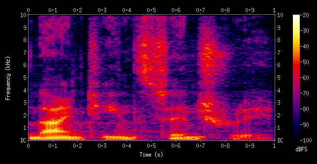
In this lecture, I’ll show you an example of feature engineering on text data.
Feature interactions and feature crosses
A feature cross is a synthetic feature formed by multiplying or crossing two or more features.
Example: Is the following dataset (XOR function) linearly separable?
import seaborn as sb
X = np.array([
    [-1, -1],
    [1, -1],
    [-1, 1],
    [1, 1]
])
y = np.array([1, 0, 0, 1])
df = pd.DataFrame(np.column_stack([X, y]), columns=["X1", "X2", "target"])
plt.figure(figsize=(4, 4))
sb.scatterplot(data=df, x="X1", y="X2", style="target", s=200, legend=False);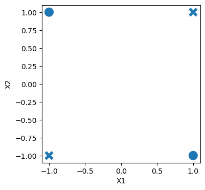
For XOR like problems, if we create a feature cross , the data becomes linearly separable.
df["X1X2"] = df["X1"] * df["X2"]
dfplt.figure(figsize=(4, 4))
sb.scatterplot(data=df, x="X2", y="X1X2", style="target", s=200, legend=False);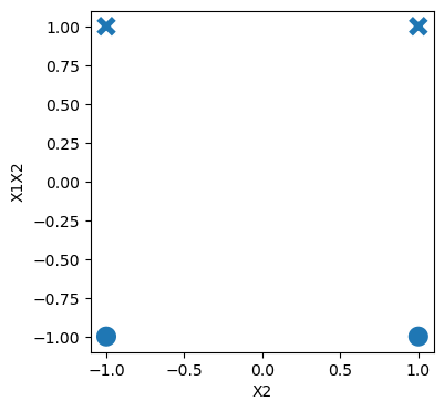
Let’s look at an example with more data points.
xx, yy = np.meshgrid(np.linspace(-3, 3, 50), np.linspace(-3, 3, 50))
rng = np.random.RandomState(0)
X_xor = rng.randn(200, 2)
y_xor = np.logical_xor(X_xor[:, 0] > 0, X_xor[:, 1] > 0)
# Interaction term
Z = X_xor[:, 0] * X_xor[:, 1]
df = pd.DataFrame({'X': X_xor[:, 0], 'Y': X_xor[:, 1], 'Z': Z, 'Class': y_xor})
df.head()plt.scatter(df[df['Class'] == True]['X'], df[df['Class'] == True]['Y'], c='blue', label='Class 0', s=50)
plt.scatter(df[df['Class'] == False]['X'], df[df['Class'] == False]['Y'], c='red', label='Class 0', s=50);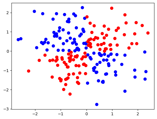
# Create an interactive 3D scatter plot using plotly
import plotly.express as px
fig = px.scatter_3d(df, x='X', y='Y', z='Z', color='Class', color_continuous_scale=['blue', 'red'])
fig.show();LogisticRegression().fit(X_xor, y_xor).score(X_xor, y_xor)0.535from sklearn.preprocessing import PolynomialFeatures
pipe_xor = make_pipeline(
PolynomialFeatures(interaction_only=True, include_bias=False), LogisticRegression()
)
pipe_xor.fit(X_xor, y_xor)
pipe_xor.score(X_xor, y_xor)0.995feature_names = (
pipe_xor.named_steps["polynomialfeatures"].get_feature_names_out().tolist()
)transformed = pipe_xor.named_steps["polynomialfeatures"].transform(X_xor)pd.DataFrame(
pipe_xor.named_steps["logisticregression"].coef_.transpose(),
index=feature_names,
columns=["Feature coefficient"],
)The interaction feature has the biggest coefficient!
Feature crosses for one-hot encoded features
You can think of feature crosses of one-hot-features as logical conjunctions
Suppose you want to predict whether you will find parking or not based on two features:
area (possible categories: UBC campus and Rogers Arena)
time of the day (possible categories: 9am and 7pm)
A feature cross in this case would create four new features:
UBC campus and 9am
UBC campus and 7pm
Rogers Arena and 9am
Rogers Arena and 7pm.
The features UBC campus and 9am on their own are not that informative but the newly created feature UBC campus and 9am or Rogers Arena and 7pm would be quite informative.
Coming up with the right combination of features requires some domain knowledge or careful examination of the data.
There is no easy way to support feature crosses in sklearn.
Demo of feature engineering with numeric features
Remember the California housing dataset we used earlier in the course?
The prediction task is predicting
median_house_valuefor a given property.
housing_df = pd.read_csv(DATA_DIR + "california_housing.csv")
housing_df.head()housing_df.info()<class 'pandas.core.frame.DataFrame'>
RangeIndex: 20640 entries, 0 to 20639
Data columns (total 10 columns):
# Column Non-Null Count Dtype
--- ------ -------------- -----
0 longitude 20640 non-null float64
1 latitude 20640 non-null float64
2 housing_median_age 20640 non-null float64
3 total_rooms 20640 non-null float64
4 total_bedrooms 20433 non-null float64
5 population 20640 non-null float64
6 households 20640 non-null float64
7 median_income 20640 non-null float64
8 median_house_value 20640 non-null float64
9 ocean_proximity 20640 non-null object
dtypes: float64(9), object(1)
memory usage: 1.6+ MB
Suppose we decide to train ridge model on this dataset.
What would happen if you train a model without applying any transformation on the categorical features ocean_proximity?
Error!! A linear model requires all features in a numeric form.
What would happen if we apply OHE on
ocean_proximitybut we do not scale the features?No syntax error. But the model results are likely to be poor.
Do we need to apply any other transformations on this data?
In this section, we will look into some common ways to do feature engineering for numeric or categorical features.
train_df, test_df = train_test_split(housing_df, test_size=0.2, random_state=123)We have total rooms and the number of households in the neighbourhood. How about creating rooms_per_household feature using this information?
train_df = train_df.assign(
    rooms_per_household=train_df["total_rooms"] / train_df["households"]
)
test_df = test_df.assign(
    rooms_per_household=test_df["total_rooms"] / test_df["households"]
)train_dfLet’s start simple. Imagine that we only three features: longitude, latitude, and our newly created rooms_per_household feature.
X_train_housing = train_df[["latitude", "longitude", "rooms_per_household"]]
y_train_housing = train_df["median_house_value"]
from sklearn.compose import make_column_transformer
numeric_feats = ["latitude", "longitude", "rooms_per_household"]
preprocessor1 = make_column_transformer(
(make_pipeline(SimpleImputer(), StandardScaler()), numeric_feats)
)lr_1 = make_pipeline(preprocessor1, Ridge())
pd.DataFrame(
cross_validate(lr_1, X_train_housing, y_train_housing, return_train_score=True)
)The scores are not great.
Let’s look at the distribution of the longitude and latitude features.
plt.figure(figsize=(6, 4), dpi=80)
plt.hist(train_df["longitude"], bins=50)
plt.title("Distribution of longitude feature");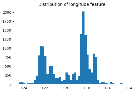
plt.figure(figsize=(6, 4), dpi=80)
plt.hist(train_df["latitude"], bins=50)
plt.title("Distribution of latitude feature");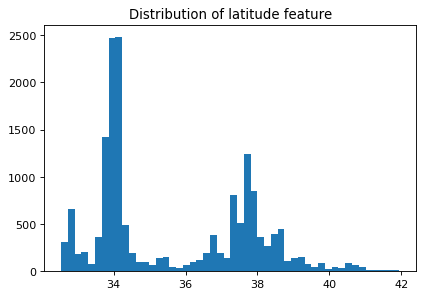
Suppose you are planning to build a linear model for housing price prediction.
If we think longitude is a good feature for prediction, does it makes sense to use the floating point representation of this feature that’s given to us?
Remember that linear models can capture only linear relationships.
How about discretizing latitude and longitude features and putting them into buckets?
This process of transforming numeric features into categorical features is called bucketing or binning.
In
sklearnyou can do this usingKBinsDiscretizertransformer.Let’s examine whether we get better results with binning.
from sklearn.preprocessing import KBinsDiscretizer

discretization_feats = ["latitude", "longitude"]
numeric_feats = ["rooms_per_household"]

preprocessor2 = make_column_transformer(
    (KBinsDiscretizer(n_bins=20, encode="onehot"), discretization_feats),
    (make_pipeline(SimpleImputer(), StandardScaler()), numeric_feats),
)
lr_2 = make_pipeline(preprocessor2, Ridge())
pd.DataFrame(
cross_validate(lr_2, X_train_housing, y_train_housing, return_train_score=True)
)The results are better with binned features. Let’s examine how do these binned features look like.
lr_2.fit(X_train_housing, y_train_housing)pd.DataFrame(
preprocessor2.fit_transform(X_train_housing).todense(),
columns=preprocessor2.get_feature_names_out(),
)How about discretizing all three features?
from sklearn.preprocessing import KBinsDiscretizer

discretization_feats = ["latitude", "longitude", "rooms_per_household"]

preprocessor3 = make_column_transformer(
    (KBinsDiscretizer(n_bins=20, encode="onehot"), discretization_feats),
)
lr_3 = make_pipeline(preprocessor3, Ridge())
pd.DataFrame(
cross_validate(lr_3, X_train_housing, y_train_housing, return_train_score=True)
)The results have improved further!!
Let’s examine the coefficients
lr_3.fit(X_train_housing, y_train_housing)feature_names = (
lr_3.named_steps["columntransformer"]
.named_transformers_["kbinsdiscretizer"]
.get_feature_names_out()
)lr_3.named_steps["ridge"].coef_.shape(60,)coefs_df = pd.DataFrame(
lr_3.named_steps["ridge"].coef_.transpose(),
index=feature_names,
columns=["coefficient"],
).sort_values("coefficient", ascending=False)
coefs_df.head<bound method NDFrame.head of coefficient
longitude_1.0 211343.036136
latitude_1.0 205059.296601
latitude_0.0 201862.534342
longitude_0.0 190319.721818
longitude_2.0 160282.191204
longitude_3.0 157234.920305
latitude_2.0 154105.963689
rooms_per_household_19.0 138503.477291
latitude_8.0 135299.516394
longitude_4.0 132292.924485
latitude_7.0 124982.236174
latitude_3.0 118563.786115
longitude_5.0 116145.526596
rooms_per_household_18.0 102044.252042
longitude_6.0 96554.525554
latitude_4.0 92809.389349
latitude_6.0 90982.951669
latitude_9.0 71096.652487
rooms_per_household_17.0 70472.564483
latitude_5.0 69411.023366
longitude_10.0 52398.892961
rooms_per_household_16.0 44311.362553
rooms_per_household_15.0 31454.877046
longitude_7.0 25658.862997
latitude_10.0 20311.784573
rooms_per_household_14.0 16460.273962
rooms_per_household_13.0 9351.210272
longitude_8.0 6322.652986
rooms_per_household_12.0 1858.970683
rooms_per_household_11.0 -12178.614567
longitude_9.0 -14579.657675
rooms_per_household_10.0 -16630.535622
rooms_per_household_9.0 -19591.810098
longitude_11.0 -22741.635200
rooms_per_household_8.0 -26919.381190
rooms_per_household_7.0 -30573.540359
rooms_per_household_6.0 -32734.570739
rooms_per_household_4.0 -40689.197649
rooms_per_household_3.0 -42060.071975
rooms_per_household_5.0 -43445.134061
rooms_per_household_2.0 -47606.596151
rooms_per_household_0.0 -50884.444297
rooms_per_household_1.0 -51143.091625
latitude_13.0 -57510.779271
longitude_14.0 -70978.802502
longitude_13.0 -89270.957075
longitude_12.0 -90669.093228
latitude_11.0 -100275.316426
longitude_15.0 -105080.071654
latitude_12.0 -111438.823543
latitude_14.0 -114836.305674
latitude_15.0 -116443.256437
longitude_16.0 -119570.316230
latitude_16.0 -140185.299164
longitude_17.0 -174766.515848
latitude_18.0 -185868.754874
latitude_17.0 -195564.951574
longitude_18.0 -205144.956966
longitude_19.0 -255751.248664
latitude_19.0 -262361.647796>Does it make sense to take feature crosses in this context?
What information would they encode?
Check out apeendixA for a demo of feature engineering on text data.
Interim summary
Feature engineering is finding the useful representation of the data that can help us effectively solve our problem.
For numeric data, some common operations to create new features are:
Discretization: Converting continuous data into discrete buckets. For example, age could be split into categories like 0-20, 21-40, etc. to learn non-linear relationships
Interaction Features: Creating new features by combining two or more existing features.
In the context of text data, if we want to go beyond bag-of-words and incorporate human knowledge in models, we carry out feature engineering. Some common features include:
ngram features
part-of-speech features
named entity features
emoticons in text
These are usually extracted from pre-trained models using libraries such as
spaCy.Now a lot of this, especially in the context of text and images, has moved to deep learning.
Despite the rise of deep learning, many industries still rely on manual feature engineering.
The best features are application-dependent.
It’s hard to give general advice. But here are some guidelines.
Ask the domain experts.
Go through academic papers in the discipline.
Often have idea of right discretization/standardization/transformation.
If no domain expert, cross-validation will help.
If you have lots of data, use deep learning methods.
The algorithms we used are very standard for Kagglers ... We spent most of our efforts in feature engineering...
- Xavier Conort, on winning the Flight Quest challenge on Kaggle
Break (5 min)

Feature selection: Introduction and motivation
With so many ways to add new features, we can increase dimensionality of the data.
More features means more complex models, which means increasing the chance of overfitting.
What is feature selection?
Find the features (columns) that are important for predicting , and remove the features that aren’t.
Given and , find the columns in that are important for predicting .
Why feature selection?
Interpretability: Models are more interpretable with fewer features. If you get the same performance with 10 features instead of 500 features, why not use the model with smaller number of features?
Computation: Models fit/predict faster with fewer columns.
Data collection: What type of new data should I collect? It may be cheaper to collect fewer columns.
Fundamental tradeoff: Can I reduce overfitting by removing useless features?
Feature selection can often result in better performing (less overfit), easier to understand, and faster model.
How do we carry out feature selection?
There are a number of ways.
You could use domain knowledge to discard features.
We are briefly going to look at two automatic feature selection methods from
sklearn:Model-based selection
Recursive feature elimination
Forward/backward selection
Very related to looking at feature importances.
from sklearn.datasets import load_breast_cancer

cancer = load_breast_cancer()
X_train, X_test, y_train, y_test = train_test_split(
    cancer.data, cancer.target, random_state=0, test_size=0.5
)X_train.shape(284, 30)pipe_lr_all_feats = make_pipeline(StandardScaler(), LogisticRegression(max_iter=1000))
pipe_lr_all_feats.fit(X_train, y_train)
pd.DataFrame(
cross_validate(pipe_lr_all_feats, X_train, y_train, return_train_score=True)
).mean()fit_time 0.001162
score_time 0.000212
test_score 0.968233
train_score 0.987681
dtype: float64Model-based selection
Use a supervised machine learning model to judge the importance of each feature.
Keep only the most important once.
Supervised machine learning model used for feature selection can be different that the one used as the final estimator.
Use a model which has some way to calculate feature importances.
To use model-based selection, we use
SelectFromModeltransformer.It selects features which have the feature importances greater than the provided threshold.
Below I’m using
RandomForestClassifierfor feature selection with threahold “median” of feature importances.Approximately how many features will be selected?
from sklearn.ensemble import RandomForestClassifier
from sklearn.feature_selection import SelectFromModel

select_rf = SelectFromModel(
    RandomForestClassifier(n_estimators=100, random_state=42),
    threshold="median"
)
Can we use KNN to select features?
from sklearn.neighbors import KNeighborsClassifier
select_knn = SelectFromModel(
    KNeighborsClassifier(),
    threshold="median"
)

pipe_lr_model_based = make_pipeline(
    StandardScaler(), select_knn, LogisticRegression(max_iter=1000)
)

#pd.DataFrame(
#    cross_validate(pipe_lr_model_based, X_train, y_train, return_train_score=True)#
#).mean()
No KNN won’t work since it does not report feature importances.
What about SVC?
select_svc = SelectFromModel(
    SVC(), threshold="median"
)

# pipe_lr_model_based = make_pipeline(
#     StandardScaler(), select_svc, LogisticRegression(max_iter=1000)
# )

# pd.DataFrame(
#    cross_validate(pipe_lr_model_based, X_train, y_train, return_train_score=True)
# ).mean()
Only with a linear kernel but not with RBF kernel
We can put the feature selection transformer in a pipeline.
pipe_lr_model_based = make_pipeline(
    StandardScaler(), select_rf, LogisticRegression(max_iter=1000)
)

pd.DataFrame(
    cross_validate(pipe_lr_model_based, X_train, y_train, return_train_score=True)
).mean()
fit_time 0.063004
score_time 0.003423
test_score 0.950564
train_score 0.974480
dtype: float64pipe_lr_model_based = make_pipeline(
StandardScaler(), select_rf, LogisticRegression(max_iter=1000)
)
pd.DataFrame(
cross_validate(pipe_lr_model_based, X_train, y_train, return_train_score=True)
).mean()fit_time 0.060543
score_time 0.003427
test_score 0.950564
train_score 0.974480
dtype: float64pipe_lr_model_based.fit(X_train, y_train)
pipe_lr_model_based.named_steps["selectfrommodel"].transform(X_train).shape(284, 15)Similar results with only 15 features instead of 30 features.
Recursive feature elimination (RFE)
Build a series of models
At each iteration, discard the least important feature according to the model.
Computationally expensive
Basic idea
fit model
find least important feature
remove
iterate.
RFE algorithm
Decide , the number of features to select.
Assign importances to features, e.g. by fitting a model and looking at
coef_orfeature_importances_.Remove the least important feature.
Repeat steps 2-3 until only features are remaining.
Note that this is not the same as just removing all the less important features in one shot!
scaler = StandardScaler()
X_train_scaled = scaler.fit_transform(X_train)
from sklearn.feature_selection import RFE
# create ranking of features
rfe = RFE(LogisticRegression(), n_features_to_select=5)
rfe.fit(X_train_scaled, y_train)
rfe.ranking_array([16, 12, 19, 13, 23, 20, 10, 1, 9, 22, 2, 25, 5, 7, 15, 4, 26,
18, 21, 8, 1, 1, 1, 6, 14, 24, 3, 1, 17, 11])print(rfe.support_)[False False False False False False False True False False False False
False False False False False False False False True True True False
False False False True False False]
print("selected features: ", cancer.feature_names[rfe.support_])selected features: ['mean concave points' 'worst radius' 'worst texture' 'worst perimeter'
'worst concave points']
How do we know what value to pass to
n_features_to_select?
Use
RFECVwhich uses cross-validation to select number of features.
from sklearn.feature_selection import RFECV

rfe_cv = RFECV(LogisticRegression(max_iter=2000), cv=10)
rfe_cv.fit(X_train_scaled, y_train)
print(rfe_cv.support_)
print(cancer.feature_names[rfe_cv.support_])
[False True False True False False True True True False True False
True True False True False False False True True True True True
False False True True False True]
['mean texture' 'mean area' 'mean concavity' 'mean concave points'
'mean symmetry' 'radius error' 'perimeter error' 'area error'
'compactness error' 'fractal dimension error' 'worst radius'
'worst texture' 'worst perimeter' 'worst area' 'worst concavity'
'worst concave points' 'worst fractal dimension']
rfe_pipe = make_pipeline(
    StandardScaler(),
    RFECV(LogisticRegression(max_iter=2000), cv=10),
    RandomForestClassifier(n_estimators=100, random_state=42),
)

pd.DataFrame(cross_validate(rfe_pipe, X_train, y_train, return_train_score=True)).mean()
fit_time 0.337034
score_time 0.001693
test_score 0.943609
train_score 1.000000
dtype: float64Slow because there is cross validation within cross validation
Not a big improvement in scores compared to all features on this toy case
(iClicker) Exercise 14.1
Select all of the following statements which are TRUE.
(A) Simple association-based feature selection approaches do not take into account the interaction between features.
(B) You can carry out feature selection using linear models by pruning the features which have very small weights (i.e., coefficients less than a threshold).
(C) The order of features removed given by
rfe.ranking_is the same as the order of original feature importances given by the model.
Warnings about feature selection
A feature is only relevant in the context of other features. Check out a
Adding/removing features can make features relevant/irrelevant.
Confounding factors can make irrelevant features the most relevant.
If features can be predicted from other other features, you cannot know which one to pick.
Relevance for features does not have a causal relationship.
Is feature selection completely hopeless?
It is messy but we still need to do it. So we try to do our best!
General advice on finding relevant features
Try forward selection.
Try other feature selection methods (e.g.,
RFE, simulated annealing, genetic algorithms)Talk to domain experts; they probably have an idea why certain features are relevant.
Don’t be overconfident.
The methods we have seen probably do not discover the ground truth and how the world really works.
They simply tell you which features help in predicting .