Lecture 12: Feature importances and model transparency¶

UBC 2025-26

Imports, LOs¶

Imports¶

Learning outcomes¶

From this lecture, students are expected to be able to:

• Interpret the coefficients of linear regression for ordinal, one-hot encoded categorical, and scaled numeric features.

• Explain why interpretability is important in ML.

• Use feature_importances_ attribute of sklearn models and interpret its output.

• Apply SHAP to assess feature importances and interpret model predictions.

• Explain force plot, summary plot, and dependence plot produced with shapely values.

I’m using seaborn in this lecture for easy heatmap plotting, which is not in the course environment. You can install it as follows.

> conda activate cpsc330
> conda install -c anaconda seaborn

Data¶

In the first part of this lecture, we’ll be using Kaggle House Prices dataset, the dataset we used in lecture 10. As usual, to run this notebook you’ll need to download the data. Unzip the data into a subdirectory called data. For this dataset, train and test have already been separated. We’ll be working with the train portion in this lecture.

• The prediction task is predicting SalePrice given features related to properties.

• Note that the target is numeric, not categorical.

Let’s separate X and y¶

Let’s identify feature types¶

Feature importances¶

• How does the output depend upon the input?

• How do the predictions change as a function of a particular feature?

• If the model is bad interpretability does not make sense.

SimpleFeature correlations¶

• Let’s look at the correlations between various features with other features and the target in our encoded data (first row/column).

• In simple terms here is how you can interpret correlations between two variables $X$ and $Y$:

  • If $Y$ goes up when $X$ goes up, we say $X$ and $Y$ are positively correlated.

  • If $Y$ goes down when $X$ goes up, we say $X$ and $Y$ are negatively correlated.

  • If $Y$ is unchanged when $X$ changes, we say $X$ and $Y$ are uncorrelated.

Let’s examine the correlations among different columns, including the target column.

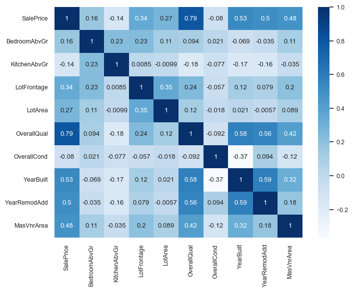
• We can immediately see that SalePrice is highly correlated with OverallQual.

• This is an early hint that OverallQual is a useful feature in predicting SalePrice.

• However, this approach is extremely simplistic.

  • It only looks at each feature in isolation.

  • It only looks at linear associations:

    • What if SalePrice is high when BsmtFullBath is 2 or 3, but low when it’s 0, 1, or 4? They might seem uncorrelated.

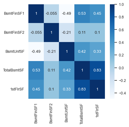
• Looking at this diagram also tells us the relationship between features.

  • For example, 1stFlrSF and TotalBsmtSF are highly correlated.

  • Do we need both of them?

  • If our model says 1stFlrSF is very important and TotalBsmtSF is very unimportant, do we trust those values?

  • Maybe TotalBsmtSF only “becomes important” if 1stFlrSF is removed.

  • Sometimes the opposite happens: a feature only becomes important if another feature is added.

Feature importances in linear models¶

• With linear regression we can look at the coefficients for each feature.

• Overall idea: predicted price = intercept + $\sum_i$ coefficient i $\times$ feature i.

Let’s look at the coefficients.

Let’s try to interpret coefficients for different types of features.

Ordinal features¶

• The ordinal features are easiest to interpret.

• Increasing by one category of exterior quality (e.g. good -> excellent) increases the predicted price by $\sim\$4195$.

  • Wow, that’s a lot!

  • Remember this is just what the model has learned. It doesn’t tell us how the world works.

Let’s perturb the example and change ExterQual to Ex.

How does the prediction change after changing ExterQual from Gd to Ex?

That’s exactly the learned coefficient for ExterQual!

So our interpretation is correct!

• Increasing by one category of exterior quality (e.g. good -> excellent) increases the predicted price by $\sim\$4195$.

Categorical features¶

• What about the categorical features?

• We have created a number of columns for each category with OHE and each category gets it’s own coefficient.

• We can talk about switching from one of these categories to another by picking a “reference” category:

• If you change the category from LandSlope_Gtl to LandSlope_Mod the prediction price goes up by $\sim\$6963$

• If you change the category from LandSlope_Gtl to LandSlope_Sev the prediction price goes down by $\sim\$8334$

Note that this might not make sense in the real world but this is what our model decided to learn given this small amount of data.

Let’s perturb the example and change LandSlope to Mod.

How does the prediction change after changing LandSlope from Gtl to Mod?

Our interpretation above is correct!

• For example, the above coefficient says that “If the roof is made of clay or tile, the predicted price is \$191K less”?

• Do we believe these interpretations??

  • Do we believe this is how the predictions are being computed? Yes.

  • Do we believe that this is how the world works? No.

Interpreting coefficients of numeric features¶

Let’s look at coefficients of PoolArea, LotFrontage, LotArea.

Intuition:

• Tricky because numeric features are scaled!

• Increasing PoolArea by 1 scaled unit increases the predicted price by $\sim\$2822$.

• Increasing LotArea by 1 scaled unit increases the predicted price by $\sim\$5109$.

• Increasing LotFrontage by 1 scaled unit decreases the predicted price by $\sim\$1578$.

Does that sound reasonable?

• For PoolArea and LotArea, yes.

• For LotFrontage, that’s surprising. Something positive would have made more sense?

It might be the case that LotFrontage is correlated with some other variable, which might have a larger positive coefficient.

BTW, let’s make sure the predictions behave as expected:

Example showing how can we interpret coefficients of scaled features.¶

• What’s one scaled unit for LotArea?

• The scaler subtracted the mean and divided by the standard deviation.

• The division actually changed the scale!

• For the unit conversion, we don’t care about the subtraction, but only the scaling.

• It seems like LotArea was divided by 8994.471032 sqft.

• The coefficient tells us that if we increase the scaled LotArea by one scaled unit the price would go up by $\approx\$5118$.

• One scaled unit represents $\sim 8994$ sqft in the original scale.

Let’s examine whether this behaves as expected.

We are expecting an increase of $5118.03516073 in the prediction compared to the original value of LotArea.

Our interpretation is correct!

• Humans find it easier to think about features in their original scale.

• How can we interpret this coefficient in the original scale?

• If I increase original LotArea by one square foot then the predicted price would go up by this amount:

Let’s perturb the example and add 1 to the LotArea.

if we add 8994.471032 to the original LotArea, the housing price prediction should go up by the coefficient 5109.35671794.

Prediction on the original example.

Prediction on the perturbed example.

• What’s the difference between predictions?

• Does the difference make sense given the coefficient of the feature?

Yes! Our interpretation is correct.

• That said don’t read too much into these coefficients without statistical training.

Interim summary¶

• Correlation among features might make coefficients completely uninterpretable.

• Fairly straightforward to interpret coefficients of ordinal features.

• In categorical features, it’s often helpful to consider one category as a reference point and think about relative importance.

• For numeric features, relative importance is meaningful after scaling.

• You have to be careful about the scale of the feature when interpreting the coefficients.

• Remember that explaining the model $\neq$ explaining the data or explaining how the world works.

• The coefficients tell us only about the model and they might not accurately reflect the data.

Transparency and explainability of ML models: Motivation¶

Activity (~5 mins)¶

Suppose you have a machine learning model which gives you a 98% cross-validation score (with the metric of your interest) and 97% test score on a reasonably sized train and test sets. Since you have impressive cross-validation and test scores, you decide to just trust the model and use it as a black box, ignoring why it’s making certain predictions.

Give some scenarios when this might or might not be problematic.

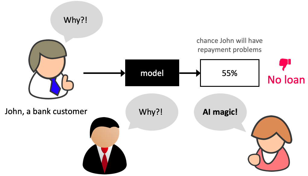
Why model transparency/interpretability?¶

• Ability to interpret ML models is crucial in many applications such as banking, healthcare, and criminal justice.

• It can be leveraged by domain experts to diagnose systematic errors and underlying biases of complex ML systems.

Source

What is model interpretability?¶

• In this lecture, our definition of model interpretability will be looking at feature importances, i.e., exploring features which are important to the model.

• There is more to interpretability than feature importances, but it’s a good start!

• Resources:

  • Interpretable Machine Learning

  • Yann LeCun, Kilian Weinberger, Patrice Simard, and Rich Caruana: Panel debate on interpretability

Data¶

• Let’s work with the adult census data set from the last lecture.

Do we have class imbalance?¶

• There is class imbalance. But without any context, both classes seem equally important.

• Let’s use accuracy as our metric.

Let’s store all the results in a dictionary called results.

We are going to use models outside sklearn. Some of them cannot handle categorical target values. So we’ll convert them to integers using LabelEncoder.

Baseline¶

Different models¶

• Logistic regression is giving reasonable scores but not the best ones.

• XGBoost and LightGBM are giving us the best CV scores.

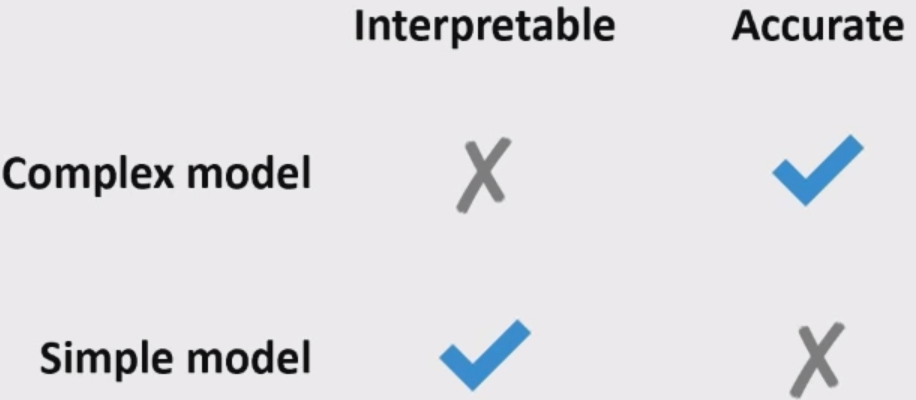
• Often simple models (e.g., linear models) are interpretable but not very accurate.

• Complex models (e.g., LightGBM) are more accurate but less interpretable.

Source

Feature importances in linear models¶

Let’s create and fit a pipeline with preprocessor and logistic regression.

• Increasing capital.gain is likely to push the prediction towards “>50k” income class

• Whereas occupation of private house service is likely to push the prediction towards “<=50K” income.

Can we get feature importances for non-linear models?

Model interpretability beyond linear models¶

• We will be looking at interpretability in terms of feature importances.

• Note that there is no absolute or perfect way to get feature importances. But it’s useful to get some idea on feature importances. So we just try our best.

We will be looking at two ways to get feature importances.

• sklearn’s feature_importances_ and permutation_importance

• SHAP

sklearn’s feature_importances_ and permutation_importance¶

Feature importance or variable importance is a score associated with a feature which tells us how “important” the feature is to the model.

Activity (~5 mins)¶

Linear models learn a coefficient associated with each feature which tells us the importance of the feature to the model.

• What might be some reasonable ways to calculate feature importances of the following models?

  • Decision trees

  • Linear SVMs

  • KNNs, RBF SVMs

• Suppose you have correlated features in your dataset. Do you need to be careful about this when you examine feature importances?

Discuss with your neighbour.

Do we have correlated features?¶

• Let’s look at columns where any correlation number is > 0.80.

• 0.80 is an arbitrary choice

Seems like there are some columns which are highly correlated.

• When we look at the feature importances, we should be mindful of these correlated features.

• Remember the limitations of looking at simple linear correlations.

• You should probably investigate multi-colinearity with more sophisticated approaches (e.g., variance inflation factors (VIF)).

sklearn’s feature_importances_ attribute vs permutation_importance¶

• Feature importances can be

  • algorithm dependent, i.e., calculated based on the information given by the model algorithm (e.g., gini importance)

  • model agnostic (e.g., by measuring increase in prediction error after permuting feature values).

• Different measures give insight into different aspects of your data and model.

Here you will find some drawbacks of using feature_importances_ attribute in the context of tree-based models.

Decision tree feature importances¶

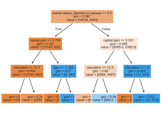
Let’s explore permutation importance.

• For each feature this method evaluates the impact of permuting feature values

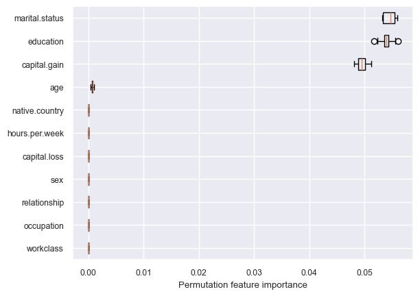
Decision tree is primarily making all decisions based on three features: marital.status, education, and capital.gain.

Let’s create and fit a pipeline with preprocessor and random forest.

Random forest feature importances¶

Which features are driving the predictions the most?

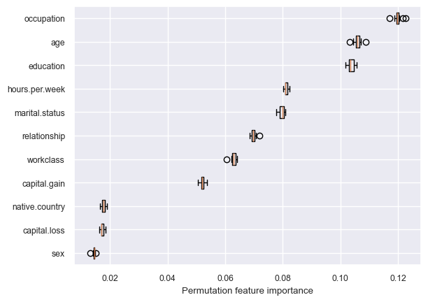
Random forest is using more features in the model compared to decision trees.

Key point¶

• Unlike the linear model coefficients, feature_importances_ do not have a sign!

  • They tell us about importance, but not an “up or down”.

  • Indeed, increasing a feature may cause the prediction to first go up, and then go down.

  • This cannot happen in linear models, because they are linear.

How can we get feature importances for non sklearn models?¶

• One way to do it is by using a tool called eli5.

Unfortunately, this is not compatible with the latest version of sklearn, which we are using.

conda install -c conda-forge eli5

• Another popular way is using SHAP. You can install it using the following in the course conda environment.

conda install -c conda-forge shap

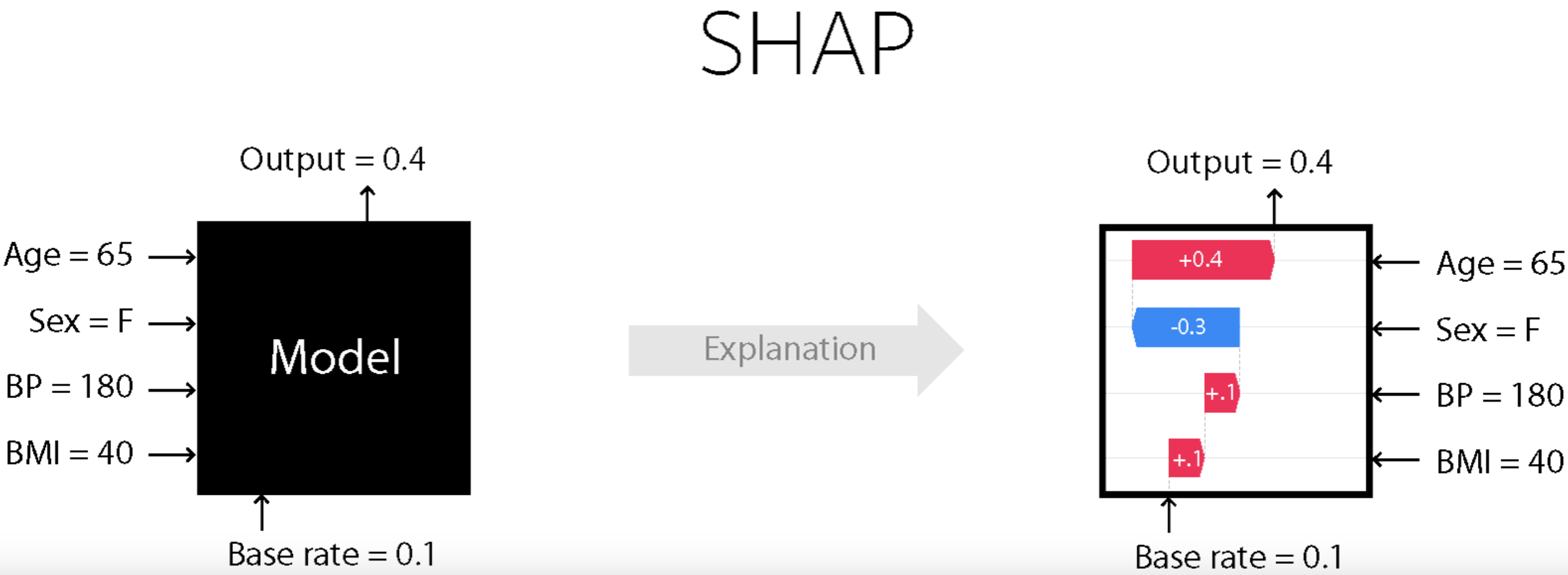
SHAP (SHapley Additive exPlanations) introduction¶

Explaining a prediction¶

Source

SHAP (SHapley Additive exPlanations) intuition

• Based on a concept from game theory called Shapley values.

• Imagine you and your friends are playing a team game where everyone contributes differently to the win. After the game, you want to figure out who contributed the most.

• Shapley values help distribute the total win fairly based on each player’s contribution.

Source

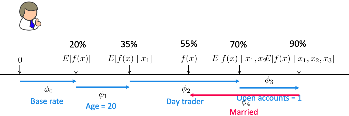
In the context of machine learning

• SHAP assigns each feature a Shapley value which tells us how much that feature pushed the model’s output higher or lower.

• A shapely value is created for each example and each feature.

• Can explain the prediction of an example by computing the contribution of each feature to the prediction.

Our focus

• How to use SHAP on our datasets to generate such plots and interpret them?

• We will be using this SHAP package.

  • Great visualizations

  • Support for different kinds of models; fast variants for tree-based models

• We are not going to discuss how SHAP works

• Check out these resources if you want to dive deeper

  • Original paper: Lundberg and Lee, 2017

  • Interpreting Machine Learning Models With SHAP

Using the SHAP package

• You should have shap in the course conda environment. If not, install it in the course conda environment.

pip install shap

or

conda install -c conda-forge shap

• Let’s try it out to explain predictions from our best performing LGBM model.

• Let’s create train and test dataframes with our transformed features.

Let’s train the model with the encoded data.

Creating SHAP values

• Let’s get SHAP values for train and test data.

• For each example and each feature, we have a SHAP value.

• SHAP values tell us how to fairly distribute the prediction among features.

SHAP plots¶

SHAP waterfall plot

• Designed to display explainations for individual predictions.

• Let’s explain the LGBM’s predictions for two examples from the test set

  • Example 1: index 10 (<=50K)

  • Example 2: index 68 (>50K)

Example 1

• The model seems quite confident about the prediction.

• If we want to know more, for example, which feature values are playing a role in this specific prediction, we can use SHAP plots.

• Remember that we have SHAP values per feature per example.

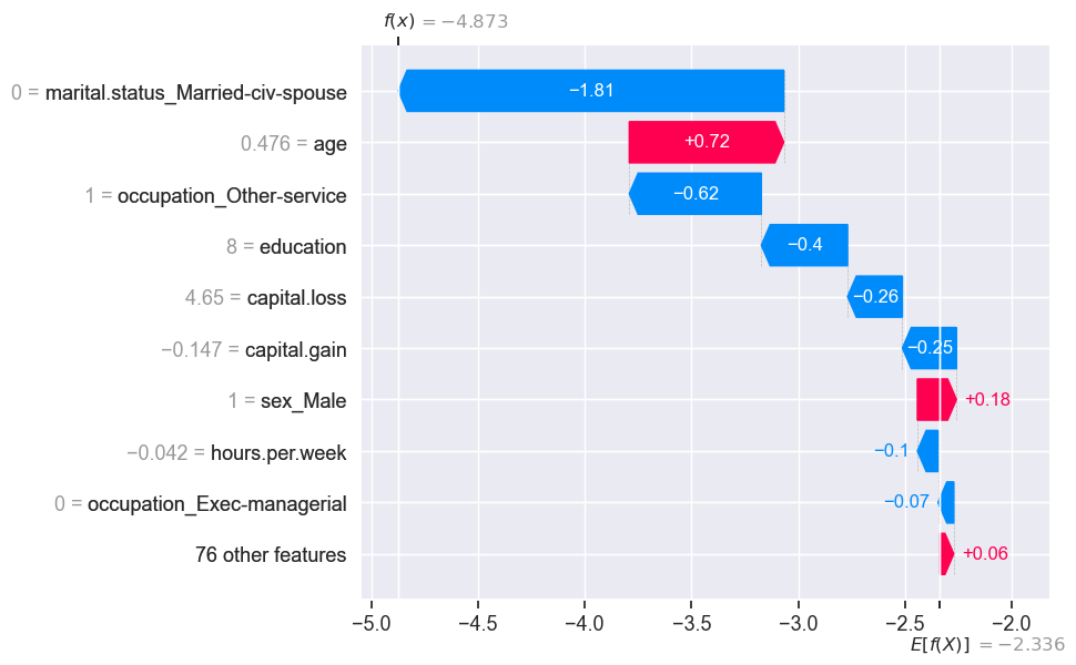
• $E[f(x)]$ is the average predicted value for all examples in our training set.

  • proportion in the context of classification

  • average in the context of regression

• $f(x)$ is the model prediction for this specific example.

• SHAP values tell us how each feature contributes to the prediction when compared to the average prediction.

• The numbers on the y-axis are feature values.

• The 76 least impactful features have been collapsed into a single term so that we don’t have too many rows. This can be changed using the max_display argument

We can get the raw model output by passing raw_score=True in predict.

What’s the raw score of the example above we are trying to explain?

• The score matches with what we see in the force plot.

• The base score above is the mean raw score. Our example has a lower raw score compared to the average raw score and the force plot tries to explain which feature values are bringing this score to a lower value.

Note: a nice thing about SHAP values is that the feature importances sum to the prediction:

Example 2

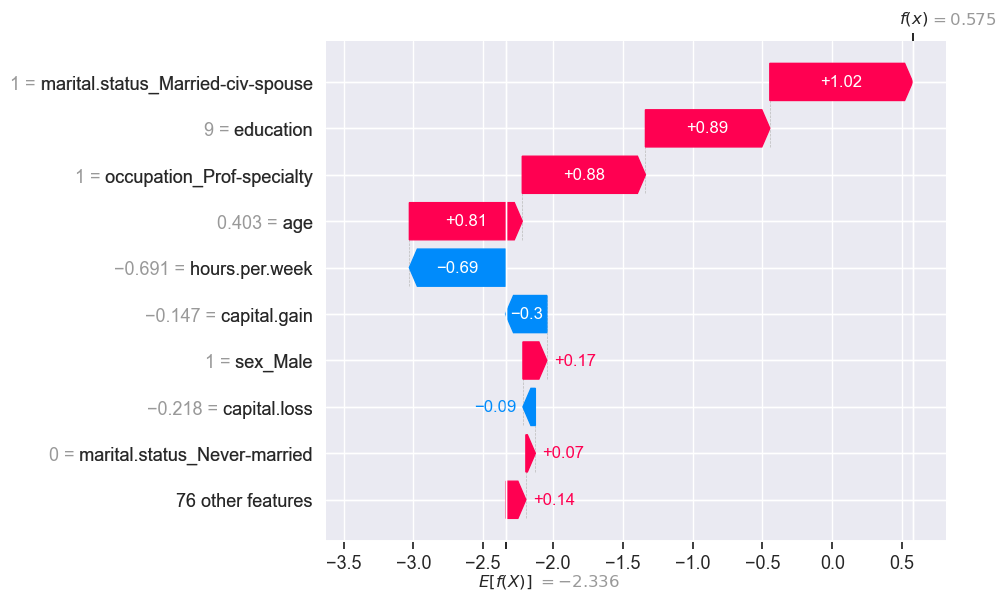
The predicted $f(x)$ is bigger than the expected $f(x)$.

SHAP Force plot

We can also display explanations of individual predictions using force plots.

SHAP: visualizing multiple predictions

• We can also visualize multiple predictions

• Let’s examine predictions of the first 4 examples from the training data.

• Let’s visualize predictions for 1,000 individuals.

SHAP summary plot

Let’s look at the average SHAP values associated with each feature.

From the documentation:

Rather than use a typical feature importance bar chart, we use a density scatter plot of SHAP values for each feature to identify how much impact each feature has on the model output for individuals in the validation dataset. Features are sorted by the sum of the SHAP value magnitudes across all samples.

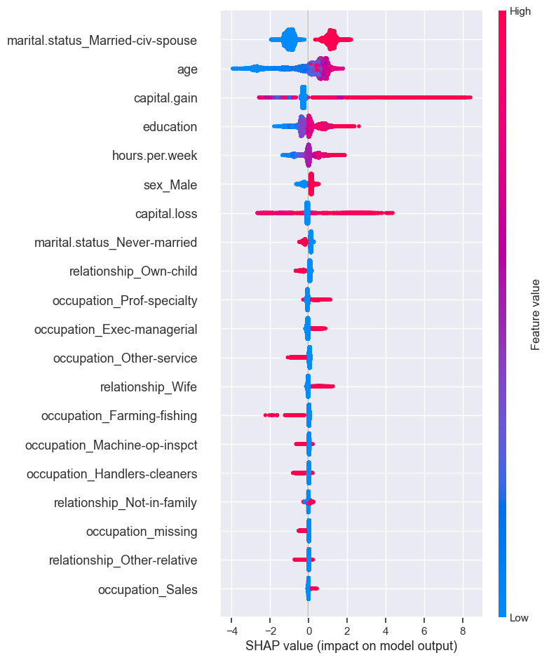
The plot shows the most important features for predicting the class. It also shows the direction of how it’s going to drive the prediction.

• Presence of the marital status of Married-civ-spouse seems to have bigger SHAP values for class 1 and absence seems to have smaller SHAP values for class 1.

• Higher levels of education seem to have bigger SHAP values for class 1 whereas smaller levels of education have smaller SHAP values.

We can also plot the summary of shap values as a bar chart.

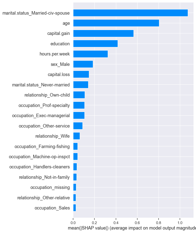
SHAP Dependence plot

From the documentation:

SHAP dependence plots show the effect of a single feature across the whole dataset. They plot a feature’s value vs. the SHAP value of that feature across many samples.

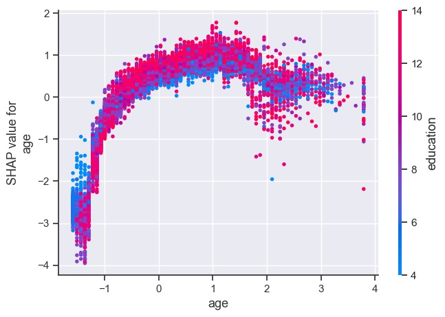
The plot above shows effect of age feature on the prediction.

• Each dot is a single prediction for examples above.

• The x-axis represents values of the feature age (scaled).

• The y-axis is the SHAP value for that feature, which represents how much knowing that feature’s value changes the output of the model for that example’s prediction.

• Lower values of age have smaller SHAP values for class “>50K”.

• Similarly, higher values of age also have a bit smaller SHAP values for class “>50K”, which makes sense.

• There is some optimal value of age between scaled age of 1 which gives highest SHAP values for for class “>50K”.

• Ignore the colour for now. The color corresponds to a second feature (education feature in this case) that may have an interaction effect with the feature we are plotting.

Here, we explore SHAP’s TreeExplainer. It also provides explainer for different kinds of models.

• TreeExplainer (supports XGBoost, CatBoost, LightGBM)

• DeepExplainer (supports deep-learning models)

• KernelExplainer (supports kernel-based models)

• GradientExplainer (supports Keras and Tensorflow models)

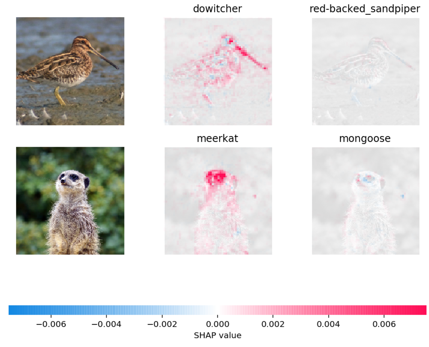
• Can also be used to explain text classification and image classification

• Example: In the picture below, red pixels represent positive SHAP values that increase the probability of the class, while blue pixels represent negative SHAP values the reduce the probability of the class.

Source

Other tools

• lime is another package.

If you’re not already impressed, keep in mind:

• So far we’ve only used sklearn models.

• Most sklearn models have some built-in measure of feature importances.

• On many tasks we need to move beyond sklearn, e.g. LightGBM, deep learning.

• These tools work on other models as well, which makes them extremely useful.

Why do we want this information?¶

Possible reasons:

• Identify features that are not useful and maybe remove them.

• Get guidance on what new data to collect.

  • New features related to useful features -> better results.

  • Don’t bother collecting useless features -> save resources.

• Help explain why the model is making certain predictions.

  • Debugging, if the model is behaving strangely.

  • Regulatory requirements.

  • Fairness / bias. See this.

  • Keep in mind this can be used on deployment predictions!

Here are some guidelines and important points to remember when you work on a prediction problem where you also want to understand which features are influencing the predictions.

• Examine multicoliniarity in your dataset using methods such as VIF.

• If you observe high correlations in your dataset, either get rid of redundant features or be mindful of these correlations during interpretation.

• Be mindful that feature relevance is not clearly defined. Adding/removing features can change feature importance/unimportance. Also, feature importances do not give us causal relationships.

• Don’t be overconfident. Always take feature importance values with a grain of salt.