Lecture 4: $k$ -Nearest Neighbours and SVM RBFs¶

UBC 2025-26

If two things are similar, the thought of one will tend to trigger the thought of the other
-- Aristotle

Imports, announcements, and LOs¶

Imports¶

import os
import sys

import IPython
import matplotlib.pyplot as plt
import numpy as np
import pandas as pd
from IPython.display import HTML

sys.path.append(os.path.join(os.path.abspath(".."), "code"))
import ipywidgets as widgets
import mglearn
from IPython.display import display
from ipywidgets import interact, interactive
from plotting_functions import *
from sklearn.dummy import DummyClassifier
from sklearn.model_selection import cross_validate, train_test_split
from utils import *

%matplotlib inline
pd.set_option("display.max_colwidth", 200)
import warnings

warnings.filterwarnings("ignore")
DATA_DIR = "../data/"

Learning outcomes¶

By the end of this lesson, you will be able to:

Explain the notion of similarity-based algorithms
Broadly describe how $k$ -NNs use distances
Discuss the effect of using a small/large value of the hyperparameter $k$ when using the $k$ -NN algorithm
Describe the problem of curse of dimensionality
Explain the general idea of SVMs with RBF kernel
Broadly describe the relation of gamma and C hyperparameters of SVMs with the fundamental tradeoff

Quick recap¶

Why do we split the data?
What are the 4 types of data splits we discussed in the last lecture?
What are the benefits of cross-validation?
What is overfitting?
What’s the fundamental trade-off in supervised machine learning?
What is the golden rule of machine learning?

Motivation and distances [video]¶

Analogy-based models¶

Suppose you are given the following training examples with corresponding labels and are asked to label a given test example.

source

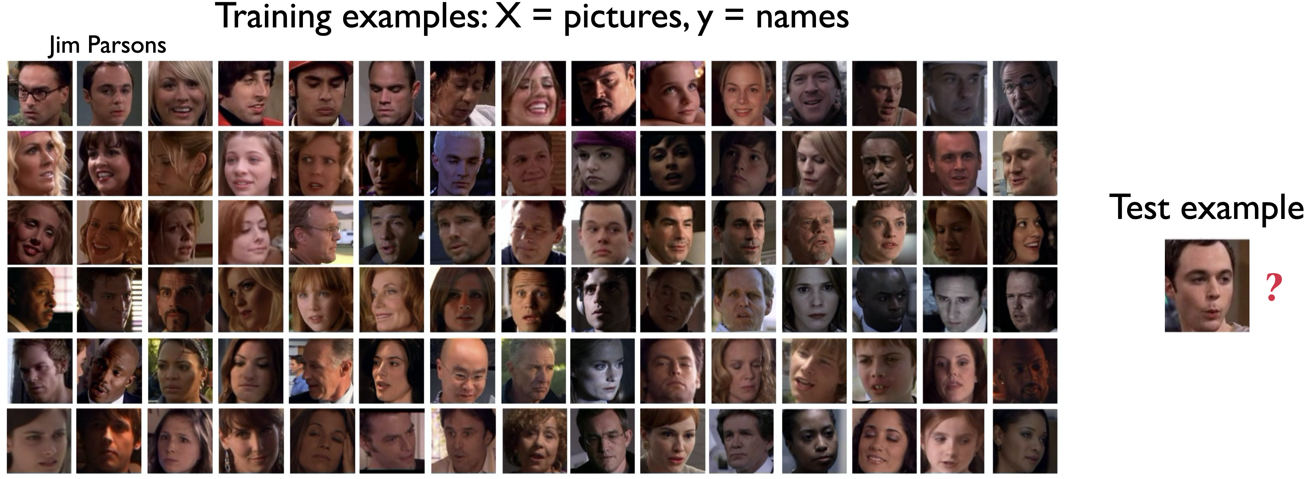
An intuitive way to classify the test example is by finding the most “similar” example(s) from the training set and using that label for the test example.

Analogy-based algorithms in practice¶

Herta’s High-tech Facial Recognition
- Feature vectors for human faces
- $k$ -NN to identify which face is on their watch list
Recommendation systems

General idea of $k$ -nearest neighbours algorithm¶

Consider the following toy dataset with two classes.
- blue circles $\rightarrow$ class 0
- red triangles $\rightarrow$ class 1
- green stars $\rightarrow$ test examples

X, y = mglearn.datasets.make_forge()
X_test = np.array([[8.2, 3.66214339], [9.9, 3.2], [11.2, 0.5]])

plot_train_test_points(X, y, X_test)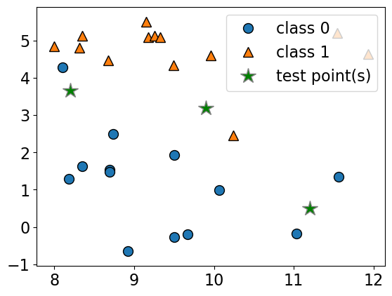

Given a new data point, predict the class of the data point by finding the “closest” data point in the training set, i.e., by finding its “nearest neighbour” or majority vote of nearest neighbours.

import matplotlib
import panel as pn
from panel import widgets
from panel.interact import interact

pn.extension()

def f(n_neighbors):
    plt.clf()
    fig = plt.figure(figsize=(6, 4))
    plot_knn_clf(X, y, X_test, n_neighbors=n_neighbors)
    plt.close()
    return pn.pane.Matplotlib(fig, tight=True)


n_neighbors_selector = pn.widgets.IntSlider(
    name="n_neighbors", start=1, end=10, value=1
)
# interact(f, n_neighbors=n_neighbors_selector)
interactive_plot = interact(f, n_neighbors=n_neighbors_selector).embed(max_opts=10)
interactive_plot

n_neighbors 1
n_neighbors 10
n_neighbors 9
n_neighbors 8
n_neighbors 7
n_neighbors 6
n_neighbors 5
n_neighbors 4
n_neighbors 3
n_neighbors 2
n_neighbors 1

<Figure size 640x480 with 0 Axes>

Geometric view of tabular data and dimensions¶

To understand analogy-based algorithms it’s useful to think of data as points in a high dimensional space.
Our X represents the problem in terms of relevant features ( $d$ ) with one dimension for each feature (column).
Examples are points in a $d$ -dimensional space.

How many dimensions (features) are there in the cities data?

cities_df = pd.read_csv(DATA_DIR + "canada_usa_cities.csv")
X_cities = cities_df[["longitude", "latitude"]]
y_cities = cities_df["country"]

mglearn.discrete_scatter(X_cities.iloc[:, 0], X_cities.iloc[:, 1], y_cities)
plt.xlabel("longitude")
plt.ylabel("latitude");

Recall the Spotify Song Attributes dataset from homework 2.
How many dimensions (features) we used in the homework?

spotify_df = pd.read_csv(DATA_DIR + "spotify.csv", index_col=0)
X_spotify = spotify_df.drop(columns=["target", "song_title", "artist"])
print("The number of features in the Spotify dataset: %d" % X_spotify.shape[1])
X_spotify.head()

The number of features in the Spotify dataset: 13

Dimensions in ML problems¶

In ML, usually we deal with high dimensional problems where examples are hard to visualize.

$d \approx 20$ is considered low dimensional
$d \approx 1000$ is considered medium dimensional
$d \approx 100,000$ is considered high dimensional

Feature vectors¶

Feature vector: is composed of feature values associated with an example.

Some example feature vectors are shown below.

print(
    "An example feature vector from the cities dataset: %s"
    % (X_cities.iloc[0].to_numpy())
)
print(
    "An example feature vector from the Spotify dataset: \n%s"
    % (X_spotify.iloc[0].to_numpy())
)

An example feature vector from the cities dataset: [-130.0437   55.9773]
An example feature vector from the Spotify dataset: 
[ 1.02000e-02  8.33000e-01  2.04600e+05  4.34000e-01  2.19000e-02
  2.00000e+00  1.65000e-01 -8.79500e+00  1.00000e+00  4.31000e-01
  1.50062e+02  4.00000e+00  2.86000e-01]

Similarity between examples¶

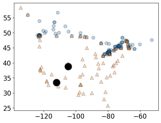
Let’s take 2 points (two feature vectors) from the cities dataset.

two_cities = X_cities.sample(2, random_state=120)
two_cities

The two sampled points are shown as big black circles.

mglearn.discrete_scatter(
    X_cities.iloc[:, 0], X_cities.iloc[:, 1], y_cities, s=8, alpha=0.3
)
mglearn.discrete_scatter(
    two_cities.iloc[:, 0], two_cities.iloc[:, 1], markers="o", c="k", s=18
);

Distance between feature vectors¶

For the cities at the two big circles, what is the distance between them?
A common way to calculate the distance between vectors is calculating the Euclidean distance.
The euclidean distance between vectors $u = <u_1, u_2, \dots, u_n>$ and $v = <v_1, v_2, \dots, v_n>$ is defined as:

distance(u, v) = \sqrt{\sum_{i =1}^{n} (u_i - v_i)^2}

(1)

Euclidean distance¶

two_cities

Subtract the two cities
Square the difference
Sum them up
Take the square root

# Subtract the two cities
print("Subtract the cities: \n%s\n" % (two_cities.iloc[1] - two_cities.iloc[0]))

# Squared sum of the difference
print(
    "Sum of squares: %0.4f" % (np.sum((two_cities.iloc[1] - two_cities.iloc[0]) ** 2))
)

# Take the square root
print(
    "Euclidean distance between cities: %0.4f"
    % (np.sqrt(np.sum((two_cities.iloc[1] - two_cities.iloc[0]) ** 2)))
)

Subtract the cities: 
longitude   -7.2488
latitude    -5.3856
dtype: float64

Sum of squares: 81.5498
Euclidean distance between cities: 9.0305

two_cities

# Euclidean distance using sklearn
from sklearn.metrics.pairwise import euclidean_distances

euclidean_distances(two_cities)

array([[0.        , 9.03049217],
       [9.03049217, 0.        ]])

Note: scikit-learn supports a number of other distance metrics.

Finding the nearest neighbour¶

Let’s look at distances from all cities to all other cities

dists = euclidean_distances(X_cities)
np.fill_diagonal(dists, np.inf)
dists.shape

(209, 209)

pd.DataFrame(dists)

Let’s look at the distances between City 0 and some other cities.

print("Feature vector for city 0: \n%s\n" % (X_cities.iloc[0]))
print("Distances from city 0 to the first 5 cities: %s" % (dists[0][:5]))
# We can find the closest city with `np.argmin`:
print(
    "The closest city from city 0 is: %d \n\nwith feature vector: \n%s"
    % (np.argmin(dists[0]), X_cities.iloc[np.argmin(dists[0])])
)

Feature vector for city 0: 
longitude   -130.0437
latitude      55.9773
Name: 0, dtype: float64

Distances from city 0 to the first 5 cities: [        inf  4.95511263  9.869531   10.10645223 10.44966612]
The closest city from city 0 is: 81 

with feature vector: 
longitude   -129.9912
latitude      55.9383
Name: 81, dtype: float64

Ok, so the closest city to City 0 is City 81.

Question¶

Why did we set the diagonal entries to infinity before finding the closest city?

Finding the distances to a query point¶

We can also find the distances to a new “test” or “query” city:

# Let's find a city that's closest to the a query city
query_point = [[-80, 25]]

dists = euclidean_distances(X_cities, query_point)
dists[0:10]

array([[58.85545875],
       [63.80062924],
       [49.30530902],
       [49.01473536],
       [48.60495488],
       [39.96834506],
       [32.92852376],
       [29.53520104],
       [29.52881619],
       [27.84679073]])

# The query point is closest to
print(
    "The query point %s is closest to the city with index %d and the distance between them is: %0.4f"
    % (query_point, np.argmin(dists), dists[np.argmin(dists)])
)

The query point [[-80, 25]] is closest to the city with index 72 and the distance between them is: 0.7982

$k$ -Nearest Neighbours ( $k$ -NNs) [video]¶

small_cities = cities_df.sample(30, random_state=90)
one_city = small_cities.sample(1, random_state=44)
small_train_df = pd.concat([small_cities, one_city]).drop_duplicates(keep=False)

X_small_cities = small_train_df.drop(columns=["country"]).to_numpy()
y_small_cities = small_train_df["country"].to_numpy()
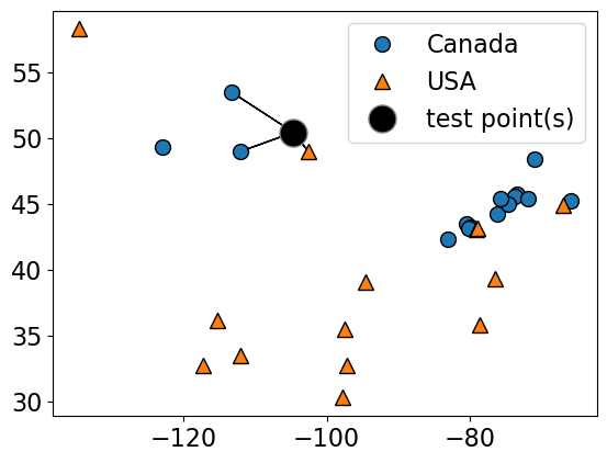
test_point = one_city[["longitude", "latitude"]].to_numpy()

plot_train_test_points(
    X_small_cities,
    y_small_cities,
    test_point,
    class_names=["Canada", "USA"],
    test_format="circle",
)

Given a new data point, predict the class of the data point by finding the “closest” data point in the training set, i.e., by finding its “nearest neighbour” or majority vote of nearest neighbours.

Suppose we want to predict the class of the black point.

An intuitive way to do this is predict the same label as the “closest” point ( $k = 1$ ) (1-nearest neighbour)
We would predict a target of USA in this case.

plot_knn_clf(
    X_small_cities,
    y_small_cities,
    test_point,
    n_neighbors=1,
    class_names=["Canada", "USA"],
    test_format="circle",
)

n_neighbors 1

How about using $k > 1$ to get a more robust estimate?

For example, we could also use the 3 closest points (k = 3) and let them vote on the correct class.
The Canada class would win in this case.

plot_knn_clf(
    X_small_cities,
    y_small_cities,
    test_point,
    n_neighbors=3,
    class_names=["Canada", "USA"],
    test_format="circle",
)

n_neighbors 3

from sklearn.neighbors import KNeighborsClassifier

k_values = [1, 3]

for k in k_values:
    neigh = KNeighborsClassifier(n_neighbors=k)
    neigh.fit(X_small_cities, y_small_cities)
    print(
        "Prediction of the black dot with %d neighbours: %s"
        % (k, neigh.predict(test_point))
    )

Prediction of the black dot with 1 neighbours: ['USA']
Prediction of the black dot with 3 neighbours: ['Canada']

Choosing `n_neighbors`¶

The primary hyperparameter of the model is n_neighbors ( $k$ ) which decides how many neighbours should vote during prediction?
What happens when we play around with n_neighbors?
Are we more likely to overfit with a low n_neighbors or a high n_neighbors?
Let’s examine the effect of the hyperparameter on our cities data.

X = cities_df.drop(columns=["country"])
y = cities_df["country"]

# split into train and test sets
X_train, X_test, y_train, y_test = train_test_split(
    X, y, test_size=0.1, random_state=123
)

k = 1
knn1 = KNeighborsClassifier(n_neighbors=k)
scores = cross_validate(knn1, X_train, y_train, return_train_score=True)
pd.DataFrame(scores)

k = 100
knn100 = KNeighborsClassifier(n_neighbors=k)
scores = cross_validate(knn100, X_train, y_train, return_train_score=True)
pd.DataFrame(scores)

plot_knn_decision_boundaries(X_train, y_train, k_values=[1, 11, 100])

How to choose `n_neighbors`?¶

n_neighbors is a hyperparameter
We can use hyperparameter optimization to choose n_neighbors.

results_dict = {
    "n_neighbors": [],
    "mean_train_score": [],
    "mean_cv_score": [],
    "std_cv_score": [],
    "std_train_score": [],
}
param_grid = {"n_neighbors": np.arange(1, 50, 5)}

for k in param_grid["n_neighbors"]:
    knn = KNeighborsClassifier(n_neighbors=k)
    scores = cross_validate(knn, X_train, y_train, return_train_score=True)
    results_dict["n_neighbors"].append(k)

    results_dict["mean_cv_score"].append(np.mean(scores["test_score"]))
    results_dict["mean_train_score"].append(np.mean(scores["train_score"]))
    results_dict["std_cv_score"].append(scores["test_score"].std())
    results_dict["std_train_score"].append(scores["train_score"].std())

results_df = pd.DataFrame(results_dict)

results_df = results_df.set_index("n_neighbors")
results_df

results_df[["mean_train_score", "mean_cv_score"]].plot();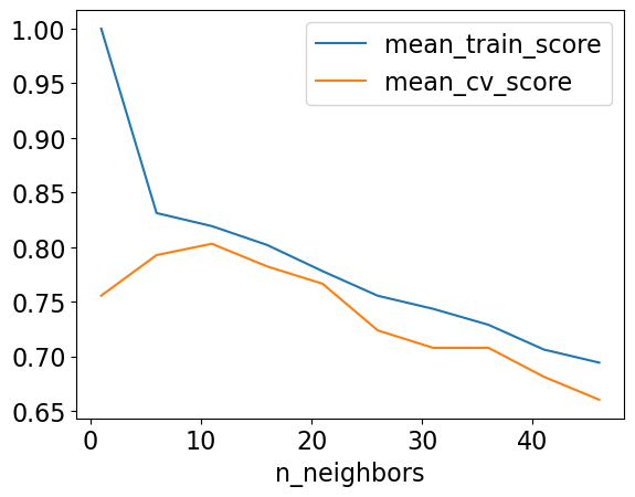

best_n_neighbours = results_df.idxmax()["mean_cv_score"]
best_n_neighbours

np.int64(11)

Let’s try our best model on test data.

knn = KNeighborsClassifier(n_neighbors=best_n_neighbours)
knn.fit(X_train, y_train)
print("Test accuracy: %0.3f" % (knn.score(X_test, y_test)))

Test accuracy: 0.905

Seems like we got lucky with the test set here.

❓❓ Questions for you¶

(iClicker) Exercise 4.1¶

Select all of the following statements which are TRUE.

(A) Analogy-based models find examples from the test set that are most similar to the query example we are predicting.
(B) Euclidean distance will always have a non-negative value.
(C) With $k$ -NN, setting the hyperparameter $k$ to larger values typically reduces training error.
(D) Similar to decision trees, $k$ -NNs finds a small set of good features.
(E) In $k$ -NN, with $k > 1$ , the classification of the closest neighbour to the test example always contributes the most to the prediction.

Break (5 min)¶

More on $k$ -NNs [video]¶

Other useful arguments of `KNeighborsClassifier`¶

weights $\rightarrow$ When predicting label, you can assign higher weight to the examples which are closer to the query example.
Exercise for you: Play around with this argument. Do you get a better validation score?

Regression with $k$ -nearest neighbours ( $k$ -NNs)¶

Can we solve regression problems with $k$ -nearest neighbours algorithm?
In $k$ -NN regression we take the average of the $k$ -nearest neighbours.
We can also have weighted regression.

See an example of regression in the lecture notes.

mglearn.plots.plot_knn_regression(n_neighbors=1)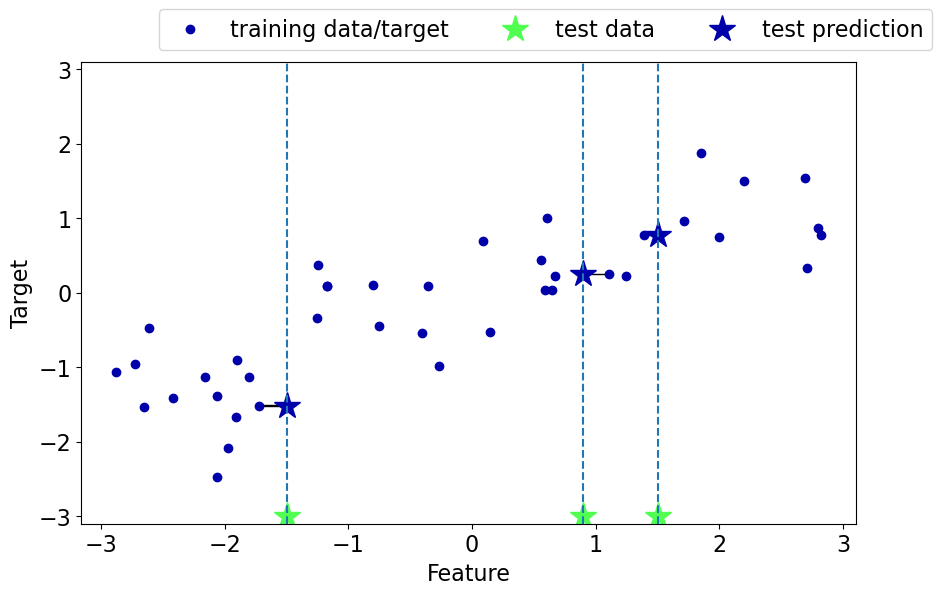

mglearn.plots.plot_knn_regression(n_neighbors=3)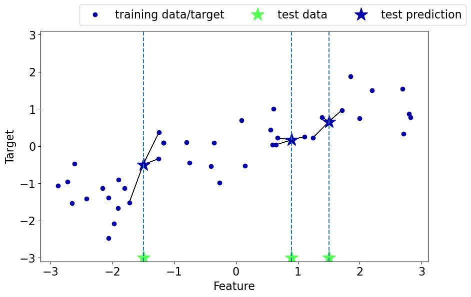

Pros of $k$ -NNs for supervised learning¶

Easy to understand, interpret.
Simple hyperparameter $k$ (n_neighbors) controlling the fundamental tradeoff.
Can learn very complex functions given enough data.
Lazy learning: Takes no time to fit

Cons of $k$ -NNs for supervised learning¶

Can be potentially be VERY slow during prediction time, especially when the training set is very large.
Often not that great test accuracy compared to the modern approaches.
It does not work well on datasets with many features or where most feature values are 0 most of the time (sparse datasets).

(Optional) Parametric vs non parametric¶

You might see a lot of definitions of these terms.
A simple way to think about this is:
- do you need to store at least $O(n)$ worth of stuff to make predictions? If so, it’s non-parametric.
Non-parametric example: $k$ -NN is a classic example of non-parametric models.
Parametric example: decision stump
If you want to know more about this, find some reading material here, here, and here.
By the way, the terms “parametric” and “non-paramteric” are often used differently by statisticians, see here for more...

Curse of dimensionality¶

Affects all learners but especially bad for nearest-neighbour.
$k$ -NN usually works well when the number of dimensions $d$ is small but things fall apart quickly as $d$ goes up.
If there are many irrelevant attributes, $k$ -NN is hopelessly confused because all of them contribute to finding similarity between examples.
With enough irrelevant attributes the accidental similarity swamps out meaningful similarity and $k$ -NN is no better than random guessing.

from sklearn.datasets import make_classification

nfeats_accuracy = {"nfeats": [], "dummy_valid_accuracy": [], "KNN_valid_accuracy": []}
for n_feats in range(4, 2000, 100):
    X, y = make_classification(n_samples=2000, n_features=n_feats, n_classes=2)
    X_train, X_test, y_train, y_test = train_test_split(
        X, y, test_size=0.2, random_state=123
    )
    dummy = DummyClassifier(strategy="most_frequent")
    dummy_scores = cross_validate(dummy, X_train, y_train, return_train_score=True)

    knn = KNeighborsClassifier()
    scores = cross_validate(knn, X_train, y_train, return_train_score=True)
    nfeats_accuracy["nfeats"].append(n_feats)
    nfeats_accuracy["KNN_valid_accuracy"].append(np.mean(scores["test_score"]))
    nfeats_accuracy["dummy_valid_accuracy"].append(np.mean(dummy_scores["test_score"]))

pd.DataFrame(nfeats_accuracy)

Support Vector Machines (SVMs) with RBF kernel [video]¶

Very high-level overview
Our goals here are
- Use scikit-learn’s SVM model.
- Broadly explain the notion of support vectors.
- Broadly explain the similarities and differences between $k$ -NNs and SVM RBFs.
- Explain how C and gamma hyperparameters control the fundamental tradeoff.

(Optional) RBF stands for radial basis functions. We won’t go into what it means in this video. Refer to this video if you want to know more.

Overview¶

Another popular similarity-based algorithm is Support Vector Machines with RBF Kernel (SVM RBFs)
Superficially, SVM RBFs are more like weighted $k$ -NNs.
- The decision boundary is defined by a set of positive and negative examples and their weights together with their similarity measure.
- A test example is labeled positive if on average it looks more like positive examples than the negative examples.

The primary difference between $k$ -NNs and SVM RBFs is that
- Unlike $k$ -NNs, SVM RBFs only remember the key examples (support vectors).
- SVMs use a different similarity metric which is called a “kernel”. A popular kernel is Radial Basis Functions (RBFs)
- They usually perform better than $k$ -NNs!

Let’s explore SVM RBFs¶

Let’s try SVMs on the cities dataset.

mglearn.discrete_scatter(X_cities.iloc[:, 0], X_cities.iloc[:, 1], y_cities)
plt.xlabel("longitude")
plt.ylabel("latitude")
plt.legend(loc=1);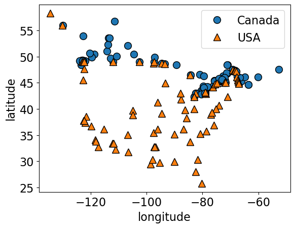

X_train, X_test, y_train, y_test = train_test_split(
    X_cities, y_cities, test_size=0.2, random_state=123
)

knn = KNeighborsClassifier(n_neighbors=best_n_neighbours)
scores = cross_validate(knn, X_train, y_train, return_train_score=True)
print("Mean validation score %0.3f" % (np.mean(scores["test_score"])))
pd.DataFrame(scores)

Mean validation score 0.803

from sklearn.svm import SVC

svm = SVC(gamma=0.01)  # Ignore gamma for now
scores = cross_validate(svm, X_train, y_train, return_train_score=True)
print("Mean validation score %0.3f" % (np.mean(scores["test_score"])))
pd.DataFrame(scores)

Mean validation score 0.820

Decision boundary of SVMs¶

We can think of SVM with RBF kernel as “smooth KNN”.

fig, axes = plt.subplots(1, 2, figsize=(16, 5))

for clf, ax in zip([knn, svm], axes):
    clf.fit(X_train, y_train)
    mglearn.plots.plot_2d_separator(
        clf, X_train.to_numpy(), fill=True, eps=0.5, ax=ax, alpha=0.4
    )
    mglearn.discrete_scatter(X_train.iloc[:, 0], X_train.iloc[:, 1], y_train, ax=ax)
    ax.set_title(clf)
    ax.set_xlabel("longitude")
    ax.set_ylabel("latitude")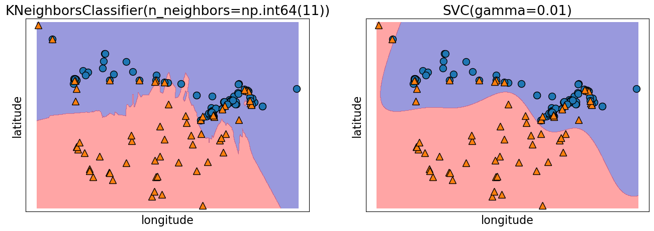

Support vectors¶

Each training example either is or isn’t a “support vector”.
- This gets decided during fit.
Main insight: the decision boundary only depends on the support vectors.
Let’s look at the support vectors.

from sklearn.datasets import make_blobs

n = 20
n_classes = 2
X_toy, y_toy = make_blobs(
    n_samples=n, centers=n_classes, random_state=300
)  # Let's generate some fake data

mglearn.discrete_scatter(X_toy[:, 0], X_toy[:, 1], y_toy)
plt.xlabel("Feature 0")
plt.ylabel("Feature 1")
svm = SVC(kernel="rbf", C=10, gamma=0.1).fit(X_toy, y_toy)
mglearn.plots.plot_2d_separator(svm, X_toy, fill=True, eps=0.5, alpha=0.4)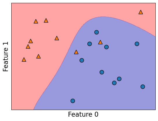

svm.support_

array([ 3, 8, 9, 14, 19, 1, 4, 6, 17], dtype=int32)

plot_support_vectors(svm, X_toy, y_toy)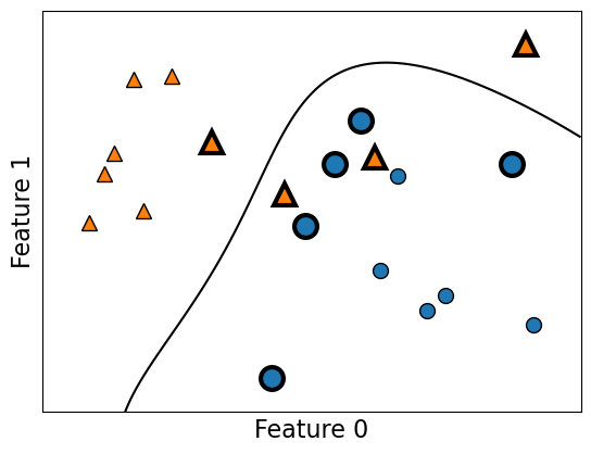

The support vectors are the bigger points in the plot above.

Hyperparameters of SVM¶

Key hyperparameters of rbf SVM are
- gamma
- C
We are not equipped to understand the meaning of these parameters at this point but you are expected to describe their relation to the fundamental tradeoff.

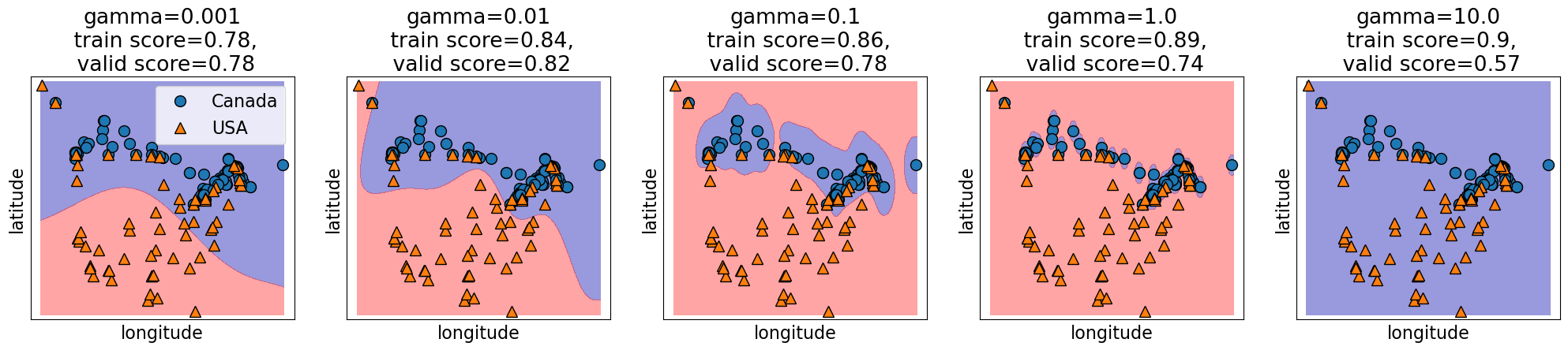
See scikit-learn’s explanation of RBF SVM parameters.

Relation of `gamma` and the fundamental trade-off¶

gamma controls the complexity (fundamental trade-off), just like other hyperparameters we’ve seen.
- larger gamma $\rightarrow$ more complex
- smaller gamma $\rightarrow$ less complex

gamma = [0.001, 0.01, 0.1, 1.0, 10.0]
plot_svc_gamma(
    gamma,
    X_train.to_numpy(),
    y_train.to_numpy(),
    x_label="longitude",
    y_label="latitude",
)

Relation of `C` and the fundamental trade-off¶

C also affects the fundamental tradeoff
- larger C $\rightarrow$ more complex
- smaller C $\rightarrow$ less complex

C = [0.1, 1.0, 100.0, 1000.0, 100000.0]
plot_svc_C(
    C, X_train.to_numpy(), y_train.to_numpy(), x_label="longitude", y_label="latitude"
)

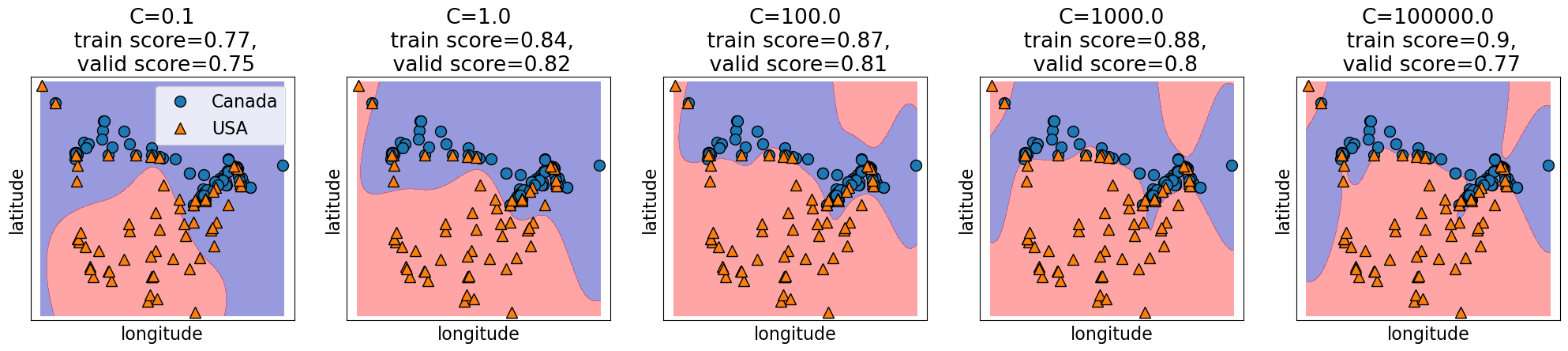
Search over multiple hyperparameters¶

So far you have seen how to carry out search over a hyperparameter
In the above case the best training error is achieved by the most complex model (large gamma, large C).
Best validation error requires a hyperparameter search to balance the fundamental tradeoff.
- In general we can’t search them one at a time.
- More on this next week. But if you cannot wait till then, you may look up the following:
  - sklearn.model_selection.GridSearchCV
  - sklearn.model_selection.RandomizedSearchCV

SVM Regressor¶

Similar to KNNs, you can use SVMs for regression problems as well.
See sklearn.svm.SVR for more details.

❓❓ Questions for you¶

(iClicker) Exercise 4.2¶

Select all of the following statements which are TRUE.

(A) $k$ -NN may perform poorly in high-dimensional space (say, d > 1000).
(B) In sklearn’s SVC classifier, large values of gamma tend to result in higher training score but probably lower validation score.
(C) If we increase both gamma and C, we can’t be certain if the model becomes more complex or less complex.

Playground¶

In this interactive playground, you will investigate how various algorithms create decision boundaries to distinguish between Iris flower species using their sepal length and width as features. By adjusting the parameters, you can observe how the decision boundaries change, which can result in either overfitting (where the model fits the training data too closely) or underfitting (where the model is too simplistic).

With k-Nearest Neighbours ( $k$ -NN), you’ll determine how many neighboring flowers to consult. Should we rely on a single nearest neighbor? Or should we consider a wider group?
With Support Vector Machine (SVM) using the RBF kernel, you’ll tweak the hyperparameters C and gamma to explore the tightrope walk between overly complex boundaries (that might overfit) and overly broad ones (that might underfit).
With Decision trees, you’ll observe the effect of max_depth on the decision boundary.

Observe the process of crafting and refining decision boundaries, one parameter at a time! Be sure to take breaks to reflect on the results you are observing.

from matplotlib.figure import Figure

from sklearn.model_selection import train_test_split
from sklearn.datasets import load_iris
from ipywidgets import interact, FloatLogSlider, IntSlider
import mglearn


# Load dataset and preprocessing
iris = load_iris(as_frame=True)
iris_df = iris.data
iris_df['species'] = iris.target
iris_df = iris_df[iris_df['species'] > 0]
X, y = iris_df[['sepal length (cm)', 'sepal width (cm)']], iris_df['species']
X_train, X_test, y_train, y_test = train_test_split(X, y, test_size=0.4, random_state=123)


# Common plot settings
def plot_results(model, X_train, y_train, title, ax):
    mglearn.plots.plot_2d_separator(model, X_train.values, fill=True, alpha=0.4, ax=ax);
    mglearn.discrete_scatter(
        X_train["sepal length (cm)"], X_train["sepal width (cm)"], y_train, s=6, ax=ax
    );
    ax.set_xlabel("sepal length (cm)", fontsize=12);
    ax.set_ylabel("sepal width (cm)", fontsize=12);
    train_score = np.round(model.score(X_train.values, y_train), 2)
    test_score = np.round(model.score(X_test.values, y_test), 2)
    ax.set_title(
        f"{title}\n train score = {train_score}\ntest score = {test_score}", fontsize=8
    );
    pass


# Widgets for SVM, k-NN, and Decision Tree
c_widget = pn.widgets.FloatSlider(
    value=1.0, start=1, end=5, step=0.1, name="C (log scale)"
)
gamma_widget = pn.widgets.FloatSlider(
    value=1.0, start=-3, end=5, step=0.1, name="Gamma (log scale)"
)
n_neighbors_widget = pn.widgets.IntSlider(
    start=1, end=40, step=1, value=5, name="n_neighbors"
)
max_depth_widget = pn.widgets.IntSlider(
    start=1, end=20, step=1, value=3, name="max_depth"
)


# The update function to create the plots
def update_plots(c, gamma=1.0, n_neighbors=5, max_depth=3):
    c_log = round(10**c, 2)  # Transform C to logarithmic scale
    gamma_log = round(10**gamma, 2)   # Transform Gamma to logarithmic scale

    fig = Figure(figsize=(8, 2))
    axes = fig.subplots(1, 3)

    models = [
        SVC(C=c_log, gamma=gamma_log, random_state=42),
        KNeighborsClassifier(n_neighbors=n_neighbors),
        DecisionTreeClassifier(max_depth=max_depth, random_state=42),
    ]
    titles = [
        f"SVM (C={c_log}, gamma={gamma_log})",
        f"k-NN (n_neighbors={n_neighbors})",
        f"Decision Tree (max_depth={max_depth})",
    ]
    for model, title, ax in zip(models, titles, axes):
        model.fit(X_train.values, y_train)
        plot_results(model, X_train, y_train, title, ax);
    # print(c, gamma, n_neighbors, max_depth)
    return pn.pane.Matplotlib(fig, tight=True);


# Bind the function to the panel widgets
interactive_plot = pn.bind(
    update_plots,
    c=c_widget.param.value_throttled,
    gamma=gamma_widget.param.value_throttled,
    n_neighbors=n_neighbors_widget.param.value_throttled,
    max_depth=max_depth_widget.param.value_throttled,
)

# Layout the widgets and the plot
dashboard = pn.Column(
    pn.Row(c_widget, n_neighbors_widget),
    pn.Row(gamma_widget, max_depth_widget),
    interactive_plot,
)

# Display the interactive dashboard
dashboard

Summary¶

We have KNNs and SVMs as new supervised learning techniques in our toolbox.
These are analogy-based learners and the idea is to assign nearby points the same label.
Unlike decision trees, all features are equally important.
Both can be used for classification or regression (much like the other methods we’ve seen).

Coming up:¶

Lingering questions:

Are we ready to do machine learning on real-world datasets?
What would happen if we use $k$ -NNs or SVM RBFs on the spotify dataset from hw2?
What happens if we have missing values in our data?
What do we do if we have features with categories or string values?

Lecture 4: k-Nearest Neighbours and SVM RBFs

Lecture 4: kkk-Nearest Neighbours and SVM RBFs¶

Imports, announcements, and LOs¶

Imports¶

Learning outcomes¶

Quick recap¶

Motivation and distances [video]¶

Analogy-based models¶

Analogy-based algorithms in practice¶

General idea of kkk-nearest neighbours algorithm¶

Geometric view of tabular data and dimensions¶

Dimensions in ML problems¶

Feature vectors¶

Similarity between examples¶

Distance between feature vectors¶

Euclidean distance¶

Finding the nearest neighbour¶

Question¶

Finding the distances to a query point¶

kkk-Nearest Neighbours (kkk-NNs) [video]¶

Choosing n_neighbors¶

How to choose n_neighbors?¶

❓❓ Questions for you¶

(iClicker) Exercise 4.1¶

Break (5 min)¶

More on kkk-NNs [video]¶

Other useful arguments of KNeighborsClassifier¶

Regression with kkk-nearest neighbours (kkk-NNs)¶

Pros of kkk-NNs for supervised learning¶

Cons of kkk-NNs for supervised learning¶

(Optional) Parametric vs non parametric¶

Curse of dimensionality¶

Support Vector Machines (SVMs) with RBF kernel [video]¶

Overview¶

Let’s explore SVM RBFs¶

Decision boundary of SVMs¶

Support vectors¶

Hyperparameters of SVM¶

Relation of gamma and the fundamental trade-off¶

Relation of C and the fundamental trade-off¶

Search over multiple hyperparameters¶

SVM Regressor¶

❓❓ Questions for you¶

(iClicker) Exercise 4.2¶

Playground¶

Summary¶

Coming up:¶

Lecture 4: $k$ -Nearest Neighbours and SVM RBFs¶

General idea of $k$ -nearest neighbours algorithm¶

$k$ -Nearest Neighbours ( $k$ -NNs) [video]¶

Choosing `n_neighbors`¶

How to choose `n_neighbors`?¶

More on $k$ -NNs [video]¶

Other useful arguments of `KNeighborsClassifier`¶

Regression with $k$ -nearest neighbours ( $k$ -NNs)¶

Pros of $k$ -NNs for supervised learning¶

Cons of $k$ -NNs for supervised learning¶

Relation of `gamma` and the fundamental trade-off¶

Relation of `C` and the fundamental trade-off¶