Week 13: Words, Words, Words

A novel is just a very long string. This week we asked: what can you compute from that string? The answer turned out to be a lot — frequency charts, character maps, sentiment arcs, named-entity networks — and the pipeline for getting there is exactly the kind of systematic data transformation you’ve been building all term. We also discovered that understanding English well enough to process it automatically is surprisingly hard, which is why spaCy exists.

Your Growing Toolkit

• Representation — how we encode meaning
• Collections — how we group things
• Control flow — how we make decisions and repeat
• Functions — how we name and reuse logic
• Abstraction — how we hide complexity
• Efficiency — how we measure cost

This week: Text as Data + NLP pipelines + Named Entity Recognition — language is messy; we build machinery to tame it!

---

Tuesday: Visualizing Literature

What Can a Novel Look Like?

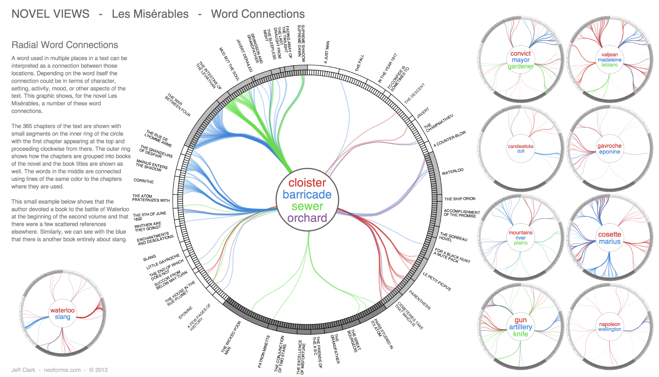
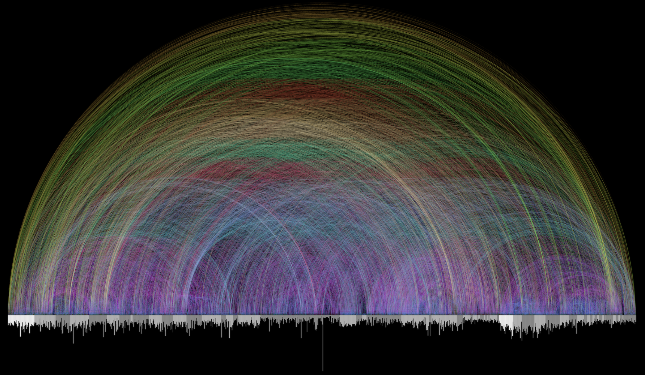
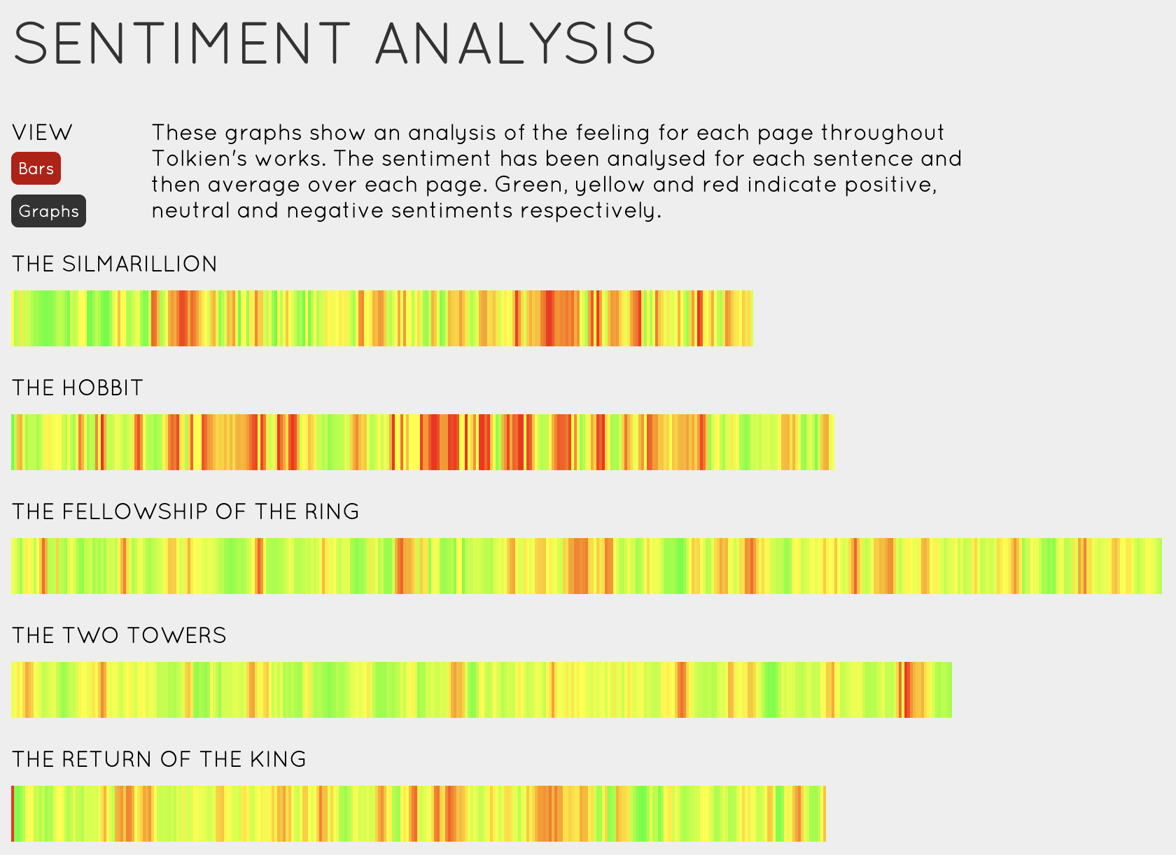
We opened with a question: if a novel is just text, what can we see in it? Researchers in computational literary studies have built some stunning visualizations that reveal structure invisible to a casual reader.

Lexical novelty across chapters and paragraphs — red = lots of new words, blue = familiar territory

Word co-occurrence: which words appear near each other most often?

Cross-references: arcs connecting mentions of the same character across a whole novel

Sentiment arc: emotional tone chapter by chapter

Geographical mapping: where does the story physically take place?

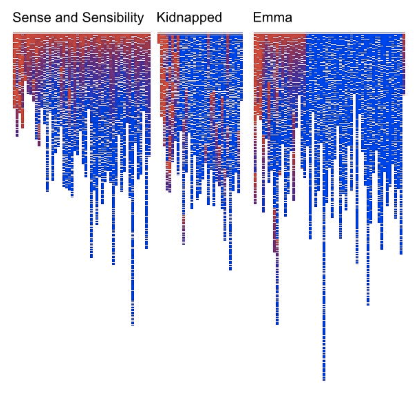
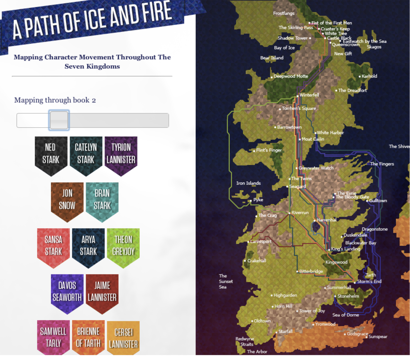
“Novels are full of new characters, new locations and new expressions. The discourse between characters involves new ideas being exchanged. We can get a hint of this by tracking the introduction of new terms in a novel.” — Matthew Hurst

---

The Text-as-Data Pipeline

A novel is just characters. Before we can do anything interesting, we need to clean and structure the text. Here’s the full pipeline:

TipFill in the blank: the six-step pipeline

1. Load the text from a .txt file into one big Python string
2. Tokenize: split into words (and punctuation, and numbers…)
3. Preprocess — four sub-steps in sequence:
   • Lowercase — unify “Valor” and “valor” into one tally
   • Remove punctuation — drop tokens that aren’t alphabetic (handles “father.”, “!”, “Dr.” correctly)
   • Remove stopwords — discard common, uninformative words (“the”, “and”, “was”) using spaCy’s curated list
   • Lemmatize — reduce words to their base form: “going” → “go”, “eaten” → “eat”, “running” → “run”
4. Count frequencies with Counter
5. Visualize as a bar chart
6. Interpret: what do the counts actually tell you about this book?

---

Watching the Pipeline Work

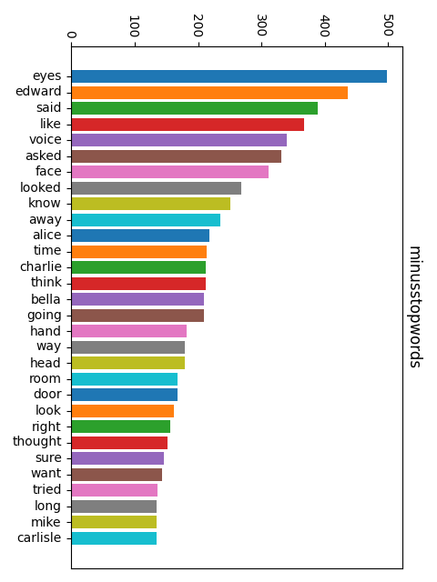
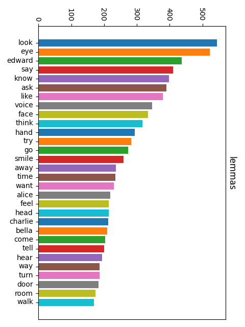
Here’s what happens to our mystery text at each stage. Each bar chart shows the 30 most common items:

Raw tokens: punctuation and capitalization dominate the top of the list

After lowercasing: “valor” and “Valor” now counted together

After removing punctuation: commas and periods are gone

After removing stopwords: meaningful words start to surface

After lemmatization: the final cleaned word frequency — now we can see what the book is actually about

ImportantWhy this order?

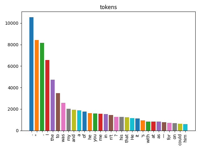
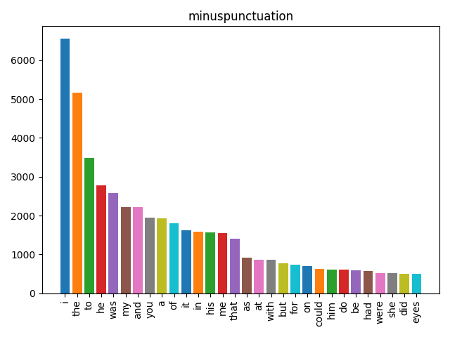
The sequence lowercase → punctuation → stopwords → lemma matters. Stopword lists are lowercase, so you must lowercase first. Lemmatization works better on clean alphabetic tokens, so remove punctuation before you lemmatize. The order isn’t arbitrary — each step prepares the data for the next.

---

Tokenization: Harder Than It Looks

Splitting “I want to go” into ['I', 'want', 'to', 'go'] seems trivial. But what about:

"Astrology. The governess was always
getting muddled with her astrolabe, and when she got specially
muddled she would take it out of the Wart by rapping his knuckles."

TipFill in the blank: tokenization result

spaCy’s tokenizer produces:

['Astrology', '.', 'The', 'governess', 'was', 'always', 'getting',
 'muddled', 'with', 'her', 'astrolabe', ',', 'and', 'when', 'she',
 'got', 'specially', 'muddled', 'she', 'would', 'take', 'it', 'out',
 'of', 'the', 'Wart', 'by', 'rapping', 'his', 'knuckles', '.']

Key insight: the period after “Astrology” is its own token — not glued to the word. The same is true of commas. This is why removing punctuation is a separate step: the tokenizer has already isolated them. And “Dr.”, “$3.50”, and “!” all work correctly because the tokenizer knows about abbreviations and special characters.

---

Stopwords: Common ≠ Useful

SpaCy comes with a list of ~300 English stopwords compiled from large corpora — words so common they add noise rather than signal: “the”, “a”, “and”, “was”, “of”, “in”, “it”, “to”, “with”…

from spacy.lang.en.stop_words import STOP_WORDS
words_without_stopwords = [w for w in words if w not in STOP_WORDS]

The more sophisticated approach is tf-idf (term frequency–inverse document frequency): instead of a fixed stopword list, it automatically downweights words that are common across all your documents. A word that appears in every book is not informative about this book.

---

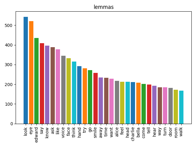
Lemmas: The Root of the Matter

A lemma is the dictionary form of a word:

Raw token	Lemma
going	go
went	go
running	run
ran	run
eaten	eat
better	good

Without lemmatization, “go”, “goes”, “going”, “went”, and “gone” each get their own tally. With lemmatization, they all count toward the same root. This gives a much more accurate picture of what ideas dominate the text.

Top 90 words after removing stopwords

Top 90 lemmas — the final cleaned vocabulary

---

Thursday: Parts of Speech + Named Entities

spaCy’s Richer Picture

Last time, we counted words. Today we went deeper: spaCy doesn’t just split your text into tokens — it understands them. When you run nlp(text), every token gets labeled with its grammatical role and its role in named entity spans.

import spacy
nlp = spacy.load("en_core_web_sm")
doc = nlp("Emma lost no time.")

[(t.text, t.pos_) for t in doc]
# → [('Emma', 'PROPN'), ('lost', 'VERB'), ('no', 'DET'), ('time', 'NOUN'), ('.', 'PUNCT')]

PROPN = proper noun — a strong signal that this token might be a named entity!

---

Parts of Speech

English words divide into two kinds:

Class	Type	Examples
Open class	New words can always be added	Noun, Verb, Adjective, Adverb
Closed class	Fixed, finite set	Preposition, Conjunction, Pronoun, Interjection

Nouns subdivide further: proper (Emma, Hartfield, London) vs common (village, house, carriage). Proper nouns are often named entities — that’s our bridge from POS tagging to NER.

---

POS Tagging is Hard: The Curling Problem

The same word can be different parts of speech depending on context. SpaCy needs to look at the whole sentence to decide:

TipFill in the blank: “curling” in three roles

• Plug in the curling iron. → adjective (JJ) — modifies “iron”
• I want to learn to play curling. → noun (NN) — the sport
• The ribbon is curling around the Maypole. → verb (VBG) — present participle

Context is everything. A word-by-word classifier would get this wrong. SpaCy uses a neural model trained on millions of sentences to disambiguate.

---

Two Levels of POS Detail

SpaCy gives you a choice of how fine-grained you want to be:

Attribute	Grain	Example values
token.pos_	Coarse (universal)	NOUN, VERB, PROPN, ADJ, ADP
token.tag_	Fine (Penn Treebank)	NN, VBD, NNP, JJ, IN

Use pos_ for most tasks; reach for tag_ when you need fine distinctions like singular vs plural noun, or past vs present tense.

---

From POS to Named Entities

POS tagging labels every token individually. But named entities are often multi-word spans: “Mr. Knightley”, “Emma Woodhouse”, “Hartfield”, “Box Hill”.

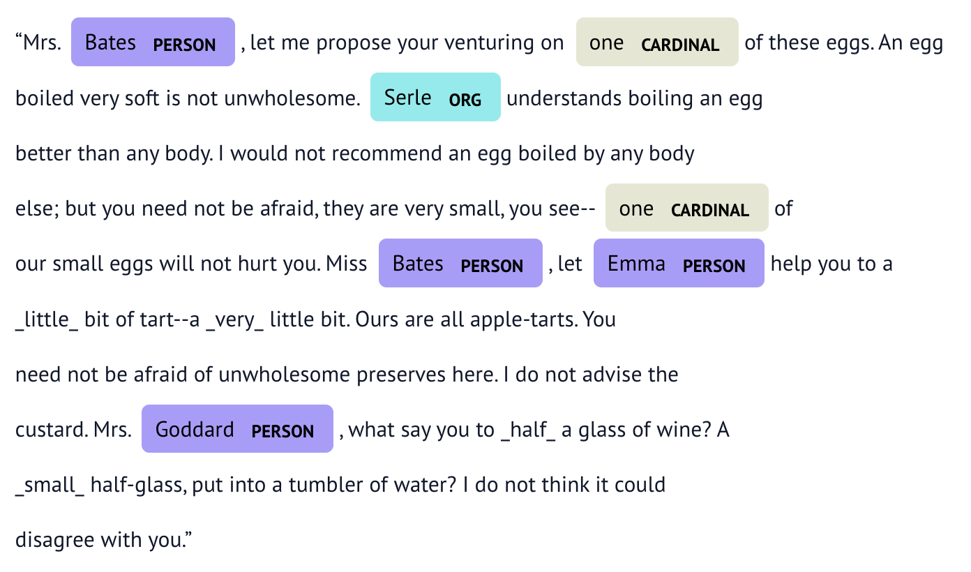
NER goes one step further: it groups runs of tokens into spans and assigns a semantic category:

Category	Meaning	Example
PERSON	People and characters	Emma Woodhouse
GPE	Geo-political entity (city, country)	London
LOC	Location (non-GPE)	Hartfield
ORG	Organization	The Crown

NER is then used to infer relationships: PERSON lives at LOCATION, PERSON meets PERSON.

SpaCy’s displacy visualizer renders named entities as colored spans directly in the text

---

IOB Encoding: Marking Entity Spans

How does spaCy mark which tokens belong to a multi-word entity? With IOB tags:

TipFill in the blank: IOB encoding

Tag	Meaning	Example
B	Beginning of an entity	('Harriet', 'B', 'PERSON')
I	Inside (continuing) an entity	('Smith', 'I', 'PERSON')
O	Outside — not part of any entity	('was', 'O', '')

So “Harriet Smith was late” becomes:

[('Harriet', 'B', 'PERSON'), ('Smith', 'I', 'PERSON'),
 ('was',     'O', ''),       ('late',  'O', '')]

The B marks the start of a span; subsequent tokens in the same span get I; everything else gets O. This lets spaCy reconstruct full multi-word names from the token stream.

---

NER in Action: Exploring a Novel

The Thursday activity used ner_nb.py to run NER on a chapter from Of Kings and Fools. Here’s the progression:

TipFill in the blank: what each expression returns

doc = nlp(textRaw)   # process the whole chapter at once

sents = list(doc.sents) → a list of spaCy Span objects, one per sentence

sentWords = [[token.text for token in sent] for sent in sents] → a list of lists of strings — each inner list is one sentence broken into words

sentWordsPOS = [[(token.text, token.pos_) for token in sent] for sent in sents] → same structure, but each word is paired with its POS tag

ents_by_sent = [[(ent.text, ent.label_) for ent in sent.ents] for sent in sents] → for each sentence, a list of (entity_text, entity_type) pairs — only named entity tokens, not plain words

sentWordsNER = [[(token.text, token.ent_iob_, token.ent_type_) for token in sent] for sent in sents] → every token, annotated with its IOB tag and entity type (empty string for O tokens)

names = [ent.text for ent in doc.ents if ent.label_ == "PERSON"] → a flat list of every person-name mention in the whole chapter

---

Character Frequency: Who’s in This Book?

Once you have all the person mentions, you can count them:

from collections import Counter
name_counts = Counter(names)
top30 = dict(name_counts.most_common(30))

The result is a frequency table of character mentions — essentially a cast list ranked by how much screen time each character gets. This is exactly the kind of insight that would take hours to compile by hand but runs in seconds computationally.

The activity also hinted at what’s coming in Week 14:

persons_by_sent = [
    [ent.text for ent in sent.ents if ent.label_ == "PERSON"]
    for sent in sents
]

This groups characters by sentence — and when two characters appear in the same sentence, that’s evidence they interact. Build a graph where characters are vertices and co-appearances are edges, and you have a social network inferred from text.

The research paper that inspired this approach — inferring social networks from literature

---

What’s Next?

In Week 14 we build on this: using NER to find all the character co-occurrences in a novel and draw the resulting social network as a graph. The pipeline is: text → NER → co-occurrence counting → graph → visualization. You’ve now seen every piece of that pipeline.

And then it’s the last class of the term — which means it’s time to talk about the bigger picture of what you’ve built this semester and what to do with it next.