Programming, problem solving, and algorithms

CPSC 203, 2026 W1

October 27, 2026

Announcements

  • Examlet 3 this Thursday through Monday.
  • Lab 7 (in-place list manipulation) and POTW 7 (numpy arrays) due Sunday.
  • Project 2 (Game of Life) released, due Monday November 16.
  • Final exam:
    • Booking opens Tuesday December 1.
    • Slots available Tuesday December 15 through Saturday December 19 (inclusive).
  • Feeling overwhelmed? You are not alone!

Voronoi Diagrams (continued)

Reminder: Queue-Based Algorithm for Voronoi Art
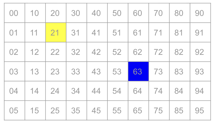
Grid with each pixel numbered, pixel 63 highlighted blue, pixel 21 highlighted yellow.

  • enqueue the centers
  • while the queue is not empty:
    • v = dequeue
    • for each valid neighbor w of v:
      • process w
      • enqueue w

Demo

Open last lecture’s activity. We’ll finish implementing the queue-based version of the algorithm.

Aside: Measuring Distance and the Choice of Neighbours

How far away are the diagonal pixels?

regular distance

four neighbours

eight neighbours

Analysis (Queue-based Version)

  1. Read image: \(O(n)\)
  2. Choose centers: \(O(dn)\)
  3. Build new image:
    1. enqueue the centers.
    2. while queue not empty:
      1. \(v\) = dequeue.
      2. for each valid neighbour \(w\) of \(v\):
        • process \(w\).
        • enqueue \(w\).
  4. Write out new image: \(O(n)\)

Size of the image: \(n\)
(\(n =\) width \(\times\) height)

Density of centers: \(d\)

Number of centers: \(dn\)

Analysis Continued: The Big Picture

How does the execution time of these algorithms compare?

  • The loop-based version is \(O(dn^2)\), where \(0 < d < 1\).
  • The queue-based version is \(O((d+1)n)\).
    • We did a lot of work for each pixel removed from the queue.

General Comments on Complexity Analysis in Computer Science

When comparing two algorithms, complexity analysis in computer science emphasizes the eventual winner as the problem size grows arbitrarily large.

  • So \(O(n^2)\) is worse than \(O(n)\) regardless of the hidden constants.

Occasionally this approach proves wrong for practical problems.

  • Computational complexity of matrix multiplication of two \(n \times n\) matrices:
    • Naive / standard approach: \(O(n^3)\).
    • Strassen’s algorithm can achieve \(O(n^{\log_2 7}) \approx O(n^{2.807})\).
    • Best complexity (as of August 2026) is \((O^{2.371177})\), but is totally impractical.
  • On modern machines, memory transfer time is often the limiting factor.

Voronoi Diagram: Example of Invariant

Complexity analysis required that no pixel appear in the queue more than once.

  • Example of an invariant: A property which always holds true for an iteration of a loop, an execution of a function / method, or perhaps a whole object or program.
  • In this case:
    • We initialize a flag processed for each pixel to False.
    • We only add the centers and considered neighbour pixels to the queue.
    • We only consider neighbour pixels if processed is False.
    • We only add a center or considered neighbour pixel to the queue after we set processed to be True for that pixel.

Voronoi Diagram: What about Correctness?

No longer easy to determine if the algorithm produces the correct result or even terminates. (See voronoi_deque_failures.py in Class Activity: Voronoi Art Fast.)

  • What happens if pixels can appear more than once?
  • What happens if we do not visit every pixel?
  • Is visiting every pixel exactly once sufficient for correctness?

Proof of correctness is hard (and may be impossible)!

  • If you stick with simple patterns (such as those from CPSC 103 / 110), it may be easier to prove correctness.
  • Mutation makes correctness proofs much harder.
  • Test, test, test…

Voronoi Diagram Summary

  • Voronoi diagrams: Region which is closest to a given point.
    • Loop-based algorithm: Simple but slow.
    • Queue-based algorithm: FIFO processing “visits” each pixel just once.
  • Complexity analysis: Queues may be harder to count than loops.
  • Flood-fill algorithm:
    • Grow outward from center(s).
    • Synchronization of “outward” by a queue.
  • Preview of graphs: How do we know what to visit next?
    • Nodes and neighbours.
    • Breadth-first search.

Graph of the Internet, circa 2003.